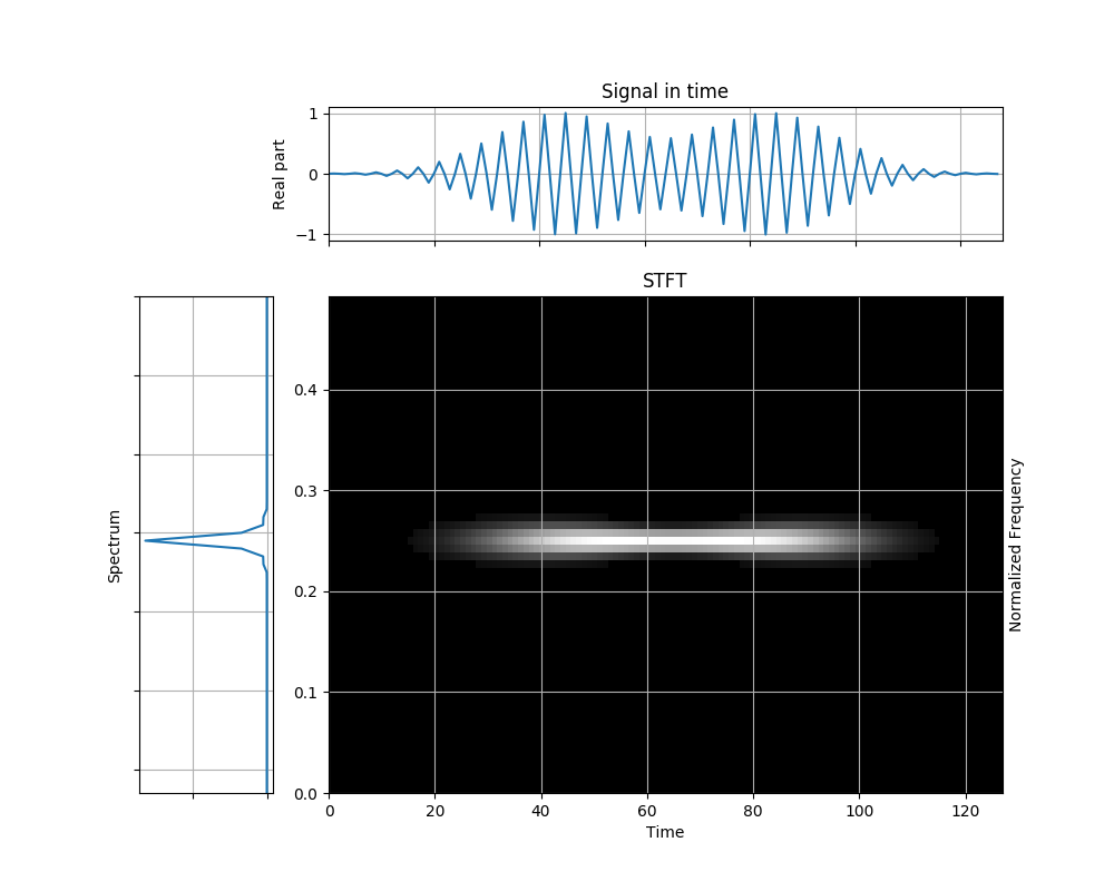
STFT of Gaussian Wave Packets with a Hamming Analysis Window

This example demonstrates the construction of a signal containing two transient components, having the same Gaussian amplitude modulation and the same frequency, but different time centers. It also shows the effect of a Hamming window function when used with th STFT.

Figure 3.7 from the tutorial.

import numpy as np
import matplotlib.pyplot as plt
from tftb.generators import atoms
from scipy.signal import hamming
from tftb.processing.linear import ShortTimeFourierTransform

coords = np.array([[45, .25, 32, 1], [85, .25, 32, 1]])
sig = atoms(128, coords)
x = np.real(sig)
window = hamming(65)
stft = ShortTimeFourierTransform(sig, n_fbins=128, fwindow=window)
stft.run()
stft.plot(show_tf=True, cmap=plt.cm.gray)