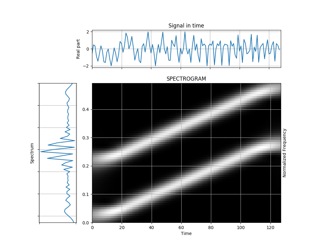
Distant Chirps with a Long Gaussian Analysis Window

This example visualizes a spectrogram of two chirp signals which are well separated in frequency ranges. A longer Gaussian analysis window suffices here to see the separation of frequencies, since the variation in frequencies is relatively slow.

Figure 3.18 from the tutorial.

from tftb.generators import fmlin
from tftb.processing.cohen import Spectrogram
import numpy as np
import matplotlib.pyplot as plt

sig = fmlin(128, 0, 0.3)[0] + fmlin(128, 0.2, 0.5)[0]
window = np.exp(np.log(0.005) * np.linspace(-1, 1, 63) ** 2)
spec = Spectrogram(sig, fwindow=window, n_fbins=128)
spec.run()
spec.plot(show_tf=True, cmap=plt.cm.gray)