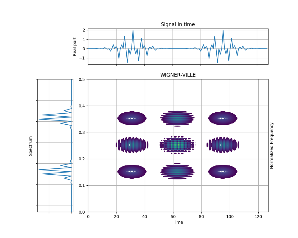
Wigner-Ville Distribution of Gaussian Atoms

This example shows the WV distribution of four Gaussian atoms, each localized at the corner of a rectangle in the time-frequency plane. The distribution does show the four signal terms, as well as six interference terms.

Figure 4.4 from the tutorial.

import numpy as np
from tftb.generators import atoms
from tftb.processing import WignerVilleDistribution

x = np.array([[32, .15, 20, 1],
             [96, .15, 20, 1],
             [32, .35, 20, 1],
             [96, .35, 20, 1]])
g = atoms(128, x)
spec = WignerVilleDistribution(g)
spec.run()
spec.plot(kind="contour", show_tf=True, scale="log")