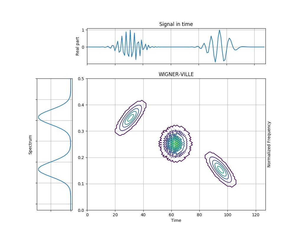
Wigner-Ville Distribution of Chirps with Different Slopes

This example demonstrates the Wigner-Ville distribution of a signal composed of two chirps with Gaussian amplitude modulation but havind linear frequency modulations with different slopes. Note that the AF interference terms are located away from the origin. We can see the two distint signal terms, but there is some interference around the middle.

Figure 4.12 from the tutorial.

from tftb.generators import fmlin, amgauss
from tftb.processing import WignerVilleDistribution
import numpy as np

n_points = 64
sig1 = fmlin(n_points, 0.2, 0.5)[0] * amgauss(n_points)
sig2 = fmlin(n_points, 0.3, 0)[0] * amgauss(n_points)
sig = np.hstack((sig1, sig2))

tfr = WignerVilleDistribution(sig)
tfr.run()
tfr.plot(kind='contour', show_tf=True)