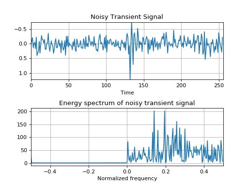
Example 2: Noisy Transient Signal
The second introductory example is a transient signal embedded in a -5 dB white gaussian noise. This transient signal is a constant frequency modulated by a one-sided exponential amplitude. The signal and its spectrum are generated as follows:
>>> import numpy as np >>> import matplotlib.pyplot as plt >>> from tftb.generators import amexpos, fmconst, sigmerge, noisecg >>> >>> # Generate a noisy transient signal. >>> transsig = amexpos(64, kind='unilateral') * fmconst(64)[0] >>> signal = np.hstack((np.zeros((100,)), transsig, np.zeros((92,)))) >>> signal = sigmerge(signal, noisecg(256), -5) >>> fig, ax = plt.subplots(2, 1) >>> ax1, ax2 = ax >>> ax1.plot(np.real(signal)) >>> ax1.grid() >>> ax1.set_title('Noisy Transient Signal') >>> ax1.set_xlabel('Time') >>> ax1.set_xlim((0, 256)) >>> ax1.set_ylim((np.real(signal).max(), np.real(signal.min()))) >>> >>> # Energy spectrum of the signal >>> dsp = np.fft.fftshift(np.abs(np.fft.fft(signal)) ** 2) >>> ax2.plot(np.arange(-128, 128, dtype=float) / 256, dsp) >>> ax2.set_title('Energy spectrum of noisy transient signal') >>> ax2.set_xlabel('Normalized frequency') >>> ax2.grid() >>> ax2.set_xlim(-0.5, 0.5) >>> >>> plt.subplots_adjust(hspace=0.5) >>> >>> plt.show()(Source code, png, hires.png, pdf)

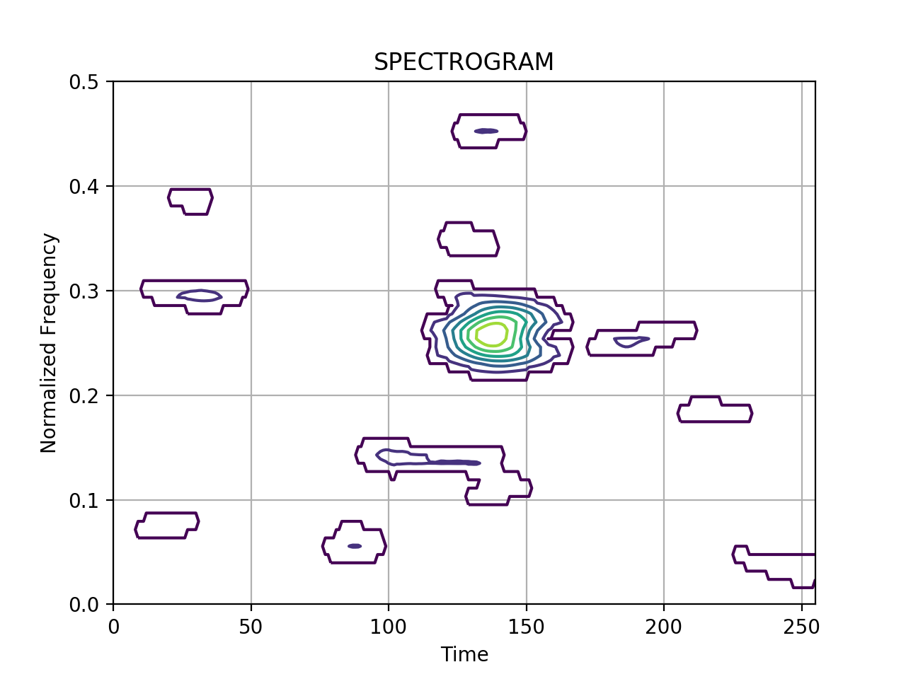
From these representations, it is difficult to localize precisely the signal in the time-domain as well as in the frequency domain. Now let us have a look at the spectrogram of this signal:
>>> from scipy.signal import hamming >>> from tftb.processing import Spectrogram >>> fwindow = hamming(65) >>> spec = Spectrogram(signal, n_fbins=128, fwindow=fwindow) >>> spec.run() >>> spec.plot(kind="contour", threshold=0.1, show_tf=False)(Source code, png, hires.png, pdf)

the transient signal appears distinctly around the normalized frequency 0.25, and between time points 125 and 160.