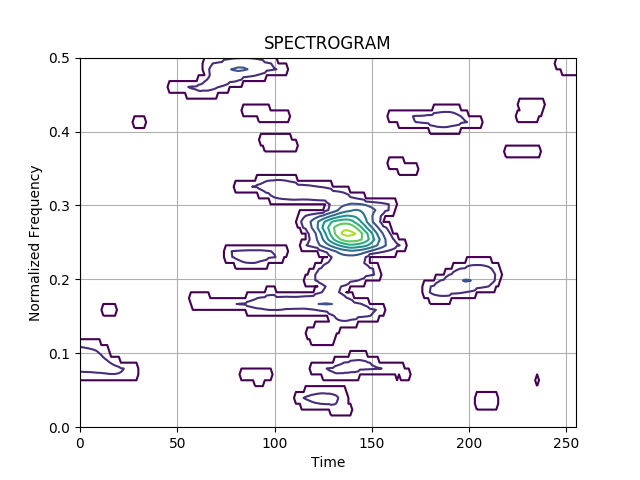
Spectrogram of a Noisy Transient Signal

This example demonstrates the simple use of a Spectrogram to localize a signal in time and frequency. The transient signal appears at the normalized frequency 0.25 and between time points 125 and 160.

Figure 1.11 from the tutorial.

import numpy as np
from scipy.signal import hamming
from tftb.generators import amexpos, fmconst, sigmerge, noisecg
from tftb.processing.cohen import Spectrogram

# Generate a noisy transient signal.
transsig = amexpos(64, kind='unilateral') * fmconst(64)[0]
signal = np.hstack((np.zeros((100,)), transsig, np.zeros((92,))))
signal = sigmerge(signal, noisecg(256), -5)

fwindow = hamming(65)
spec = Spectrogram(signal, n_fbins=128, fwindow=fwindow)
spec.run()
spec.plot(kind="contour", threshold=0.1, show_tf=False)