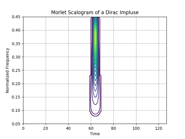
Morlet Scalogram of a Dirac Impulse

This example plots the scalogram of a Dirac impulse functions. This shows the behaviour of the scalograms as the scale (or inversely, the frequency) changes. it is well localized for small scales (large frequencies), and less localized as the scale increases (as the frequency decreases).

Figure 3.19 from the tutorial.

from tftb.generators import anapulse
from tftb.processing import Scalogram
import numpy as np
import matplotlib.pyplot as plt

sig1 = anapulse(128)
tfr, t, f, _ = Scalogram(sig1, waveparams=6, fmin=0.05, fmax=0.45,
                         n_voices=128).run()
tfr = np.abs(tfr) ** 2
threshold = np.amax(tfr) * 0.05
tfr[tfr <= threshold] = 0.0
t, f = np.meshgrid(t, f)
plt.contour(t, f, tfr, 20)
plt.grid()
plt.title('Morlet Scalogram of a Dirac Impluse')
plt.xlabel('Time')
plt.ylabel('Normalized Frequency')
plt.show()