Instantatneous Frequency and Group Delay Estimation of a Multi-Component Nonstationary Signal

Figure 2.10 from the tutorial.

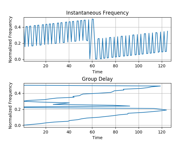
#  N=128; x1=fmlin(N,0,0.2); x2=fmlin(N,0.3,0.5);
#  x=x1+x2;
#  ifr=instfreq(x); subplot(211); plot(ifr);
#  fn=0:0.01:0.5; gd=sgrpdlay(x,fn);
#  subplot(212); plot(gd,fn);
from tftb.generators import fmlin
from tftb.processing import inst_freq, group_delay
import matplotlib.pyplot as plt
import numpy as np

N = 128
x1, _ = fmlin(N, 0, 0.2)
x2, _ = fmlin(N, 0.3, 0.5)
x = x1 + x2
ifr = inst_freq(x)[0]
fn = np.arange(0.51, step=0.01)
gd = group_delay(x, fn)

plt.subplot(211)
plt.plot(ifr)
plt.xlim(1, N)
plt.grid(True)
plt.title('Instantaneous Frequency')
plt.xlabel('Time')
plt.ylabel('Normalized Frequency')

plt.subplot(212)
plt.plot(gd, fn)
plt.xlim(1, N)
plt.grid(True)
plt.title('Group Delay')
plt.xlabel('Time')
plt.ylabel('Normalized Frequency')

plt.subplots_adjust(hspace=0.5)

plt.show()