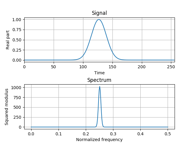
Heisenbeg-Gabor Inequality

This example demonstrates the Heisenberg-Gabor inequality.

Simply put, the inequality states that the time-bandwidth product of a signal is lower bound by some constant (in this case normalized to unity). This means that a signal cannot have arbitrarily high precision in time and frequency simultaneously.

Figure 2.2 from the tutorial.

Out:

Time Center: 126.99999999999999
Time Duration: 31.999999999999996
Frequency Center: 4.336808689942018e-19
Frequency Spreading: 0.03125
Time-bandwidth product: 0.9999999999999999

from tftb.generators import amgauss
from tftb.processing import loctime, locfreq
import numpy as np
import matplotlib.pyplot as plt

# generate signal
signal = amgauss(256)
plt.subplot(211), plt.plot(np.real(signal))
plt.xlim(0, 256)
plt.xlabel('Time')
plt.ylabel('Real part')
plt.title('Signal')
plt.grid()
fsig = np.fft.fftshift(np.abs(np.fft.fft(signal)) ** 2)
plt.subplot(212), plt.plot(np.linspace(0, 0.5, 256), fsig)
plt.xlabel('Normalized frequency')
plt.ylabel('Squared modulus')
plt.title('Spectrum')
plt.grid()
plt.subplots_adjust(hspace=0.5)
plt.show()

tm, T = loctime(signal)
print("Time Center: {}".format(tm))
print("Time Duration: {}".format(T))
fm, B = locfreq(signal)
print("Frequency Center: {}".format(fm))
print("Frequency Spreading: {}".format(B))
print("Time-bandwidth product: {}".format(T * B))