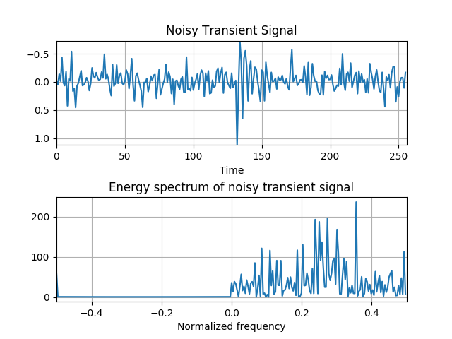
Spectrum of a Noisy Transient Signal

This example shows how to generate a noisy transient signal with the following characteristics:

• One-sided exponential amplitude modulation (See amexpos)
• Constant frequency modulation (See fmconst)
• -5 dB complex gaussian noise (See noisecg and sigmerge)

And how to plot its energy spectrum.

Figure 1.10 of the tutorial.

import numpy as np
import matplotlib.pyplot as plt
from tftb.generators import amexpos, fmconst, sigmerge, noisecg

# Generate a noisy transient signal.
transsig = amexpos(64, kind='unilateral') * fmconst(64)[0]
signal = np.hstack((np.zeros((100,)), transsig, np.zeros((92,))))
signal = sigmerge(signal, noisecg(256), -5)
fig, ax = plt.subplots(2, 1)
ax1, ax2 = ax
ax1.plot(np.real(signal))
ax1.grid()
ax1.set_title('Noisy Transient Signal')
ax1.set_xlabel('Time')
ax1.set_xlim((0, 256))
ax1.set_ylim((np.real(signal).max(), np.real(signal.min())))

# Energy spectrum of the signal
dsp = np.fft.fftshift(np.abs(np.fft.fft(signal)) ** 2)
ax2.plot(np.arange(-128, 128, dtype=float) / 256, dsp)
ax2.set_title('Energy spectrum of noisy transient signal')
ax2.set_xlabel('Normalized frequency')
ax2.grid()
ax2.set_xlim(-0.5, 0.5)

plt.subplots_adjust(hspace=0.5)

plt.show()