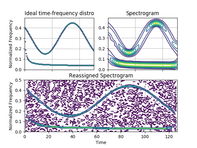
Comparison of a Spectrogram and a Reassigned Spectrogram

This example compares the spectrogram and the reassigned spectrogram of a hybrid signal (containing sinusoidal, constant and linear frequency modulations), against its ideal time-frequency characteristics.

Figure 4.34 from the tutorial.

Out:

/home/docs/checkouts/readthedocs.org/user_builds/tftb/envs/latest/lib/python3.7/site-packages/tftb/processing/reassigned.py:542: ComplexWarning: Casting complex values to real discards the imaginary part
  rtfr[int(jcolhat), int(icolhat) - 1] += tfr[jcol, icol]
/home/docs/checkouts/readthedocs.org/user_builds/tftb/envs/latest/lib/python3.7/site-packages/numpy/ma/core.py:2786: ComplexWarning: Casting complex values to real discards the imaginary part
  order=order, subok=True, ndmin=ndmin)

from tftb.generators import fmsin, fmhyp
from tftb.processing import ideal_tfr, reassigned_spectrogram, Spectrogram
import numpy as np
import matplotlib.pyplot as plt

n_points = 128
sig1, if1 = fmsin(n_points, 0.15, 0.45, 100, 1, 0.4, -1)
sig2, if2 = fmhyp(n_points, [1, .5], [32, 0.05])
sig = sig1 + sig2
ideal, t, f = ideal_tfr(np.vstack((if1, if2)))
_, re_spec, _ = reassigned_spectrogram(sig)
spec, t3, f3 = Spectrogram(sig).run()

# Ideal tfr
plt.subplot(221)
plt.contour(t, f, ideal, 1)
plt.grid(True)
plt.gca().set_xticklabels([])
plt.title("Ideal time-frequency distro")
plt.ylabel('Normalized Frequency')

# Spectrogram
plt.subplot(222)
plt.contour(t3, f3[:64], spec[:64, :])
plt.grid(True)
plt.gca().set_xticklabels([])
plt.title("Spectrogram")

# Reassigned Spectrogram
plt.subplot(212)
f = np.linspace(0, 0.5, 64)
plt.contour(np.arange(128), f, re_spec[:64, :])
plt.grid(True)
plt.title("Reassigned Spectrogram")
plt.xlabel('Time')
plt.ylabel('Normalized Frequency')

plt.show()