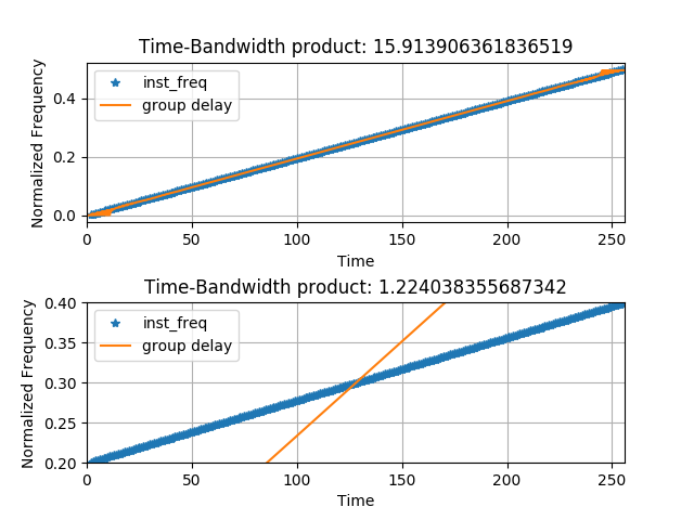
Comparison of Instantaneous Frequency and Group Delay

Instantaneous frequency and group delay are very closely related. The former is the frequency of a signal at a given instant, and the latter is the time delay of frequency components. As this example shows, they coincide with each other for a given signal when the time bandwidth product of the signal is sufficiently high.

Figure 2.5 from the tutorial.

import numpy as np
import matplotlib.pyplot as plt
from tftb.generators import amgauss, fmlin
from tftb.processing import loctime, locfreq, inst_freq, group_delay

time_instants = np.arange(2, 256)
sig1 = amgauss(256, 128, 90) * fmlin(256)[0]
tm, T1 = loctime(sig1)
fm, B1 = locfreq(sig1)
ifr1 = inst_freq(sig1, time_instants)[0]
f1 = np.linspace(0, 0.5 - 1.0 / 256, 256)
gd1 = group_delay(sig1, f1)

plt.subplot(211)
plt.plot(time_instants, ifr1, '*', label='inst_freq')
plt.plot(gd1, f1, '-', label='group delay')
plt.xlim(0, 256)
plt.grid(True)
plt.legend()
plt.title("Time-Bandwidth product: {0}".format(T1 * B1))
plt.xlabel('Time')
plt.ylabel('Normalized Frequency')


sig2 = amgauss(256, 128, 30) * fmlin(256, 0.2, 0.4)[0]
tm, T2 = loctime(sig2)
fm, B2 = locfreq(sig2)
ifr2 = inst_freq(sig2, time_instants)[0]
f2 = np.linspace(0.02, 0.4, 256)
gd2 = group_delay(sig2, f2)


plt.subplot(212)
plt.plot(time_instants, ifr2, '*', label='inst_freq')
plt.plot(gd2, f2, '-', label='group delay')
plt.ylim(0.2, 0.4)
plt.xlim(0, 256)
plt.grid(True)
plt.legend()
plt.title("Time-Bandwidth product: {0}".format(T2 * B2))
plt.xlabel('Time')
plt.ylabel('Normalized Frequency')

plt.subplots_adjust(hspace=0.5)

plt.show()