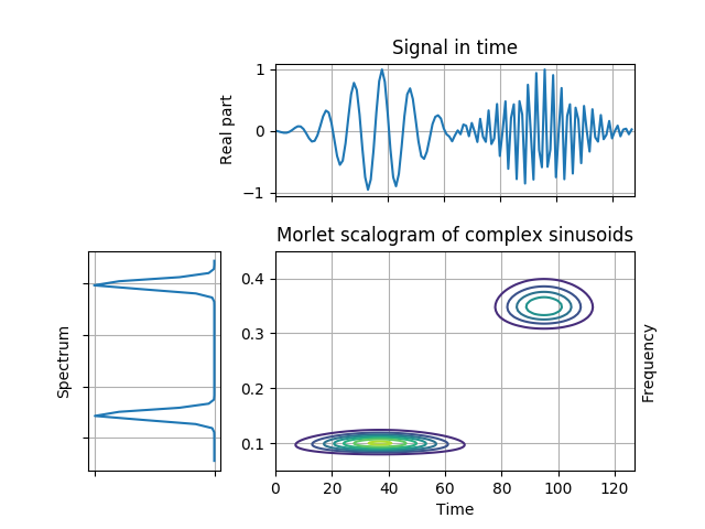
Morlet Scalogram of Gaussian Atoms

This example demonstrates the effect of frequency-dependent smoothing that is accomplished in a Morlet scalogram. Note that the localization at lower frequencies is much better.

Figure 4.18 from the tutorial.

from tftb.processing import Scalogram
from tftb.generators import atoms
import numpy as np
from mpl_toolkits.axes_grid1 import make_axes_locatable
import matplotlib.pyplot as plt

sig = atoms(128, np.array([[38, 0.1, 32, 1], [96, 0.35, 32, 1]]))
tfr, t, freqs, _ = Scalogram(sig, fmin=0.05, fmax=0.45,
                             time_instants=np.arange(1, 129)).run()
t, f = np.meshgrid(t, freqs)

fig, axContour = plt.subplots()
axContour.contour(t, f, tfr)
axContour.grid(True)
axContour.set_title("Morlet scalogram of complex sinusoids")
axContour.set_ylabel('Frequency')
axContour.yaxis.set_label_position('right')
axContour.set_xlabel('Time')

divider = make_axes_locatable(axContour)
axTime = divider.append_axes("top", 1.2, pad=0.5)
axFreq = divider.append_axes("left", 1.2, pad=0.5)
axTime.plot(np.real(sig))
axTime.set_xticklabels([])
axTime.set_xlim(0, 128)
axTime.set_ylabel('Real part')
axTime.set_title('Signal in time')
axTime.grid(True)
freq_y = np.linspace(0, 0.5, sig.shape[0] / 2)
freq_x = (abs(np.fft.fftshift(np.fft.fft(sig))) ** 2)[::-1][:64]
ix = np.logical_and(freq_y >= 0.05, freq_y <= 0.45)
axFreq.plot(freq_x[ix], freq_y[ix])
# axFreq.set_ylim(0.05, 0.45)
axFreq.set_yticklabels([])
axFreq.set_xticklabels([])
axFreq.grid(True)
axFreq.set_ylabel('Spectrum')
axFreq.invert_xaxis()
axFreq.grid(True)
plt.show()