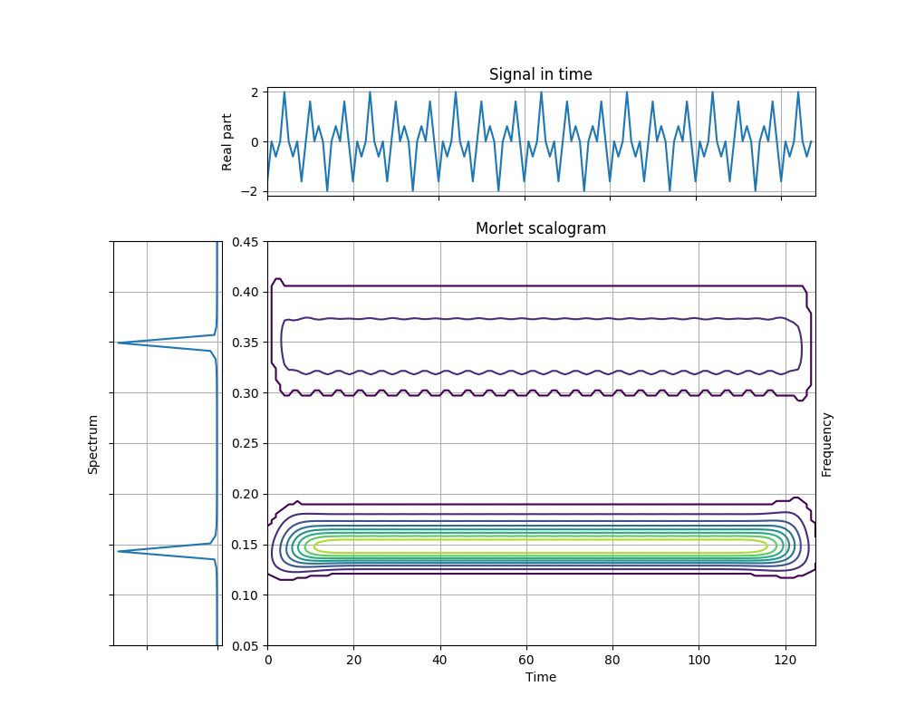
Morlet Scalogram of a Multicomponent Signal

This example demonstrates the visualization of the Morlet scalogram of a signal containing two complex sinusoids. In a scalogram, the frequency resolution varies on the scale of the signal. Here, the frequency resolution decreases at higher frequencies (lower scale).

Figure 3.20 from the tutorial.

from tftb.processing import Scalogram
from tftb.generators import fmconst
import numpy as np
from mpl_toolkits.axes_grid1 import make_axes_locatable
import matplotlib.pyplot as plt

sig2 = fmconst(128, .15)[0] + fmconst(128, .35)[0]
tfr, t, freqs, _ = Scalogram(sig2, time_instants=np.arange(1, 129), waveparams=6,
                         fmin=0.05, fmax=0.45, n_voices=128).run()
tfr = np.abs(tfr) ** 2
threshold = np.amax(tfr) * 0.05
tfr[tfr <= threshold] = 0.0
t, f = np.meshgrid(t, freqs)

fig, axContour = plt.subplots(figsize=(10, 8))
axContour.contour(t, f, tfr)
axContour.grid(True)
axContour.set_title("Morlet scalogram")
axContour.set_ylabel('Frequency')
axContour.yaxis.set_label_position('right')
axContour.set_xlabel('Time')

divider = make_axes_locatable(axContour)
axTime = divider.append_axes("top", 1.2, pad=0.5)
axFreq = divider.append_axes("left", 1.2, pad=0.5)
axTime.plot(np.real(sig2))
axTime.set_xticklabels([])
axTime.set_xlim(0, 128)
axTime.set_ylabel('Real part')
axTime.set_title('Signal in time')
axTime.grid(True)
freq_y = np.linspace(0, 0.5, sig2.shape[0] / 2)
freq_x = (abs(np.fft.fftshift(np.fft.fft(sig2))) ** 2)[::-1][:64]
axFreq.plot(freq_x, freq_y)
axFreq.set_ylim(0.05, 0.45)
axFreq.set_yticklabels([])
axFreq.set_xticklabels([])
axFreq.grid(True)
axFreq.set_ylabel('Spectrum')
axFreq.invert_xaxis()
axFreq.grid(True)
plt.show()