Note
Click here to download the full example code
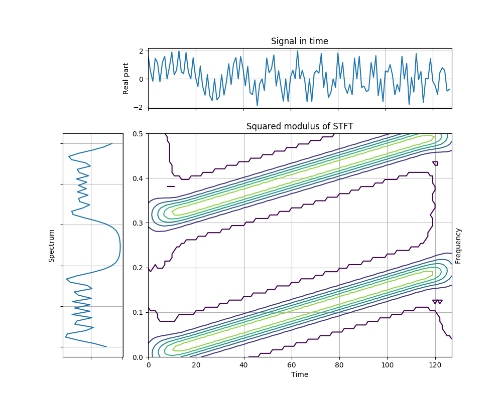
Short time Fourier transform of a multi-component nonstationary signal
Compute and visualize the STFT of a multi component nonstationary signal.
Figure 2.11 from the tutorial.
from tftb.generators import fmlin
from tftb.processing.linear import ShortTimeFourierTransform
import matplotlib.pyplot as plt
from scipy.signal import hamming
import numpy as np
from mpl_toolkits.axes_grid1 import make_axes_locatable

N = 128
x1, _ = fmlin(N, 0, 0.2)
x2, _ = fmlin(N, 0.3, 0.5)
x = x1 + x2

n_fbins = 128
window = hamming(33)
tfr, _, _ = ShortTimeFourierTransform(x, timestamps=None, n_fbins=n_fbins,
                                      fwindow=window).run()
tfr = tfr[:64, :]
threshold = np.amax(np.abs(tfr)) * 0.05
tfr[np.abs(tfr) <= threshold] = 0.0 + 1j * 0.0
tfr = np.abs(tfr) ** 2
t = np.arange(tfr.shape[1])
f = np.linspace(0, 0.5, tfr.shape[0])

T, F = np.meshgrid(t, f)

fig, axScatter = plt.subplots(figsize=(10, 8))
axScatter.contour(T, F, tfr, 5)
axScatter.grid(True)
axScatter.set_title('Squared modulus of STFT')
axScatter.set_ylabel('Frequency')
axScatter.yaxis.set_label_position("right")
axScatter.set_xlabel('Time')
divider = make_axes_locatable(axScatter)
axTime = divider.append_axes("top", 1.2, pad=0.5)
axFreq = divider.append_axes("left", 1.2, pad=0.5)
axTime.plot(np.real(x))
axTime.set_xticklabels([])
axTime.set_xlim(0, N)
axTime.set_ylabel('Real part')
axTime.set_title('Signal in time')
axTime.grid(True)
axFreq.plot((abs(np.fft.fftshift(np.fft.fft(x))) ** 2)[::-1][:64], f[:64])
axFreq.set_yticklabels([])
axFreq.set_xticklabels([])
axFreq.invert_xaxis()
axFreq.set_ylabel('Spectrum')
axFreq.grid(True)
plt.show()
Total running time of the script: ( 0 minutes 1.083 seconds)