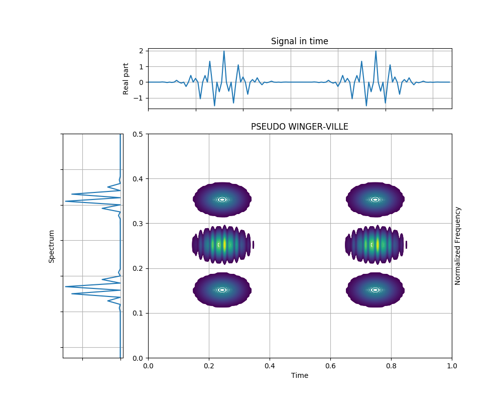
Pseudo Wigner-Ville Distribution of Gaussian Atoms

This example shows the Pseudo Wigner-Ville distribution of four Gaussian atoms located at the corners of a rectangle in the time-frequency plane. The PseudoWignerVilleDistribution class uses frequency smoothing, which attenuates the interferences oscillating along the time axis.

Figure 4.5 from the tutorial.

Out:

/home/docs/checkouts/readthedocs.org/user_builds/tftb/envs/latest/lib/python3.7/site-packages/matplotlib/contour.py:1197: ComplexWarning: Casting complex values to real discards the imaginary part
  self.levels = np.asarray(levels_arg).astype(np.float64)

import numpy as np
from tftb.generators import atoms
from tftb.processing import PseudoWignerVilleDistribution

x = np.array([[32, .15, 20, 1],
             [96, .15, 20, 1],
             [32, .35, 20, 1],
             [96, .35, 20, 1]])
g = atoms(128, x)
t = np.linspace(0, 1, 128)
spec = PseudoWignerVilleDistribution(g, timestamps=t)
spec.run()
spec.plot(kind="contour", scale="log", show_tf=True)