Wigner Ville Distribution of Analytic Gaussian Atoms

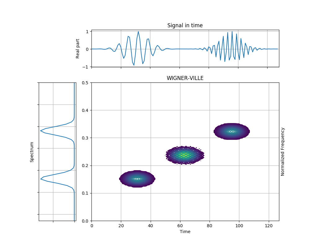
This example shows the WVD of and analytic Gaussian atom. As seen in Figure 4.6, the WVD of a real valued signal may present interference terms and spectral aliasing. One of the ways to fix this is to use an analytic signal, which divides the spectral domain into two parts: real and imaginary. Thus, the number of interference terms is also halved. Secondly, analytic signals have no negative components, so the terms present in the negative half plane also vanish.

Figure 4.7 from the tutorial.

import numpy as np
from tftb.generators import atoms
from tftb.processing import WignerVilleDistribution

x = np.array([[32, .15, 20, 1],
             [96, .32, 20, 1]])
g = atoms(128, x)
spec = WignerVilleDistribution(g)
spec.run()
spec.plot(show_tf=True, kind="contour", scale="log")