Note
Click here to download the full example code
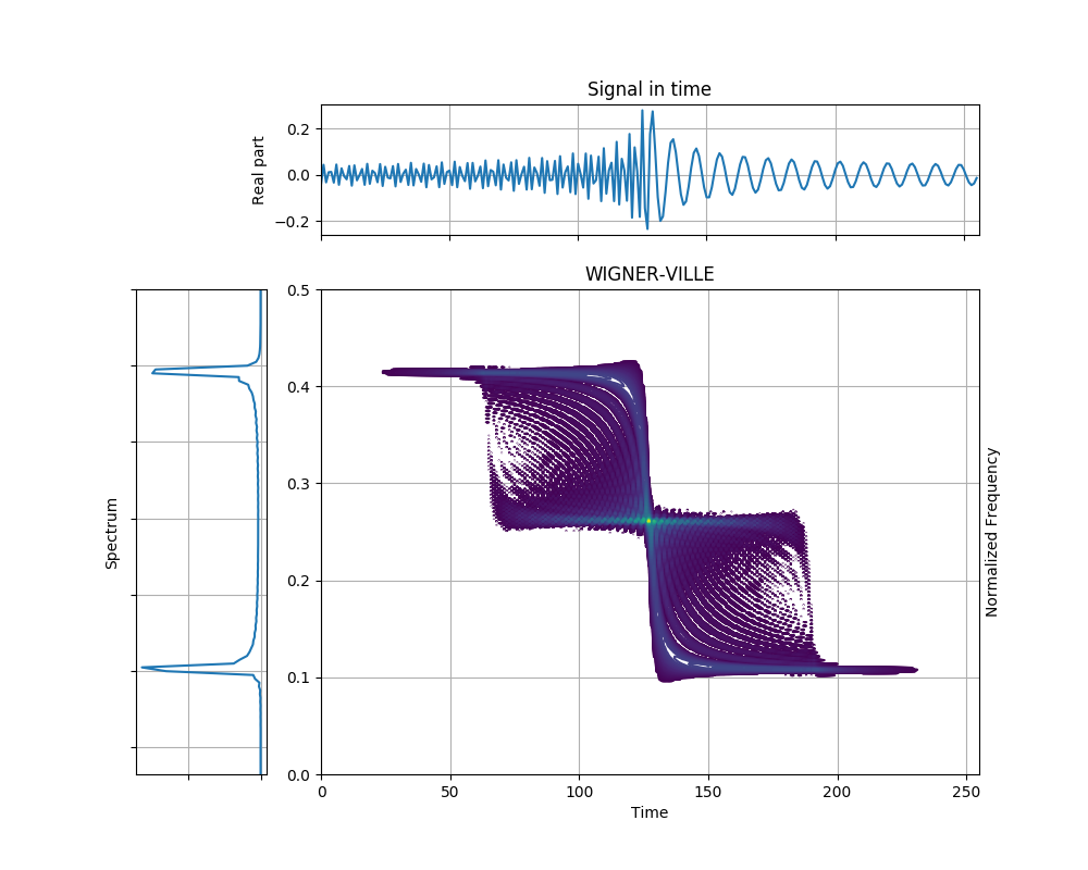
Wigner-Ville Distribution of a Doppler Signal
This example shows the Wigner-Ville distribution of a Doppler signal. The signal steadily rises and falls, but there are many interference terms present in the time-friequency plane, due to the bilinearity of the signal.
Figure 4.2 from the tutorial.
from tftb.generators import doppler
from tftb.processing import WignerVilleDistribution

fm, am, iflaw = doppler(256, 50.0, 13.0, 10.0, 200.0)
sig = am * fm
dist = WignerVilleDistribution(sig)
tfr, times, freqs = dist.run()
dist.plot(show_tf=True, kind="contour", scale="log")
Total running time of the script: ( 0 minutes 0.710 seconds)