Friedman’s Instantaneous Frequency Density Calculation

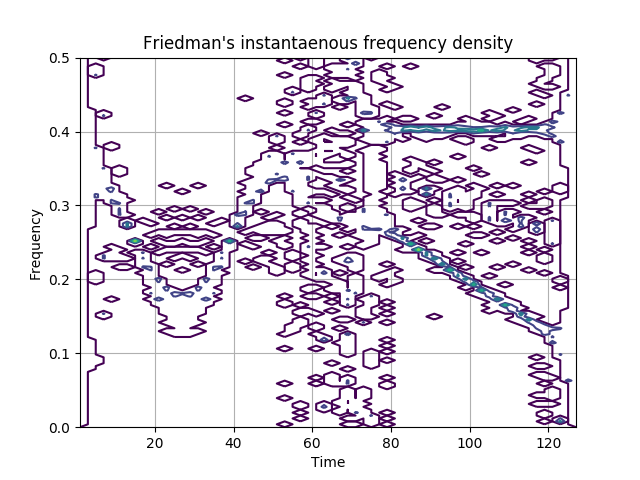
This example uses Friedman’s method to calculate the instantaneous frequency density of a hybrid signal. The method consists of computing the histograms of frequency displacements of the spectrogram of the signal.

Figure 4.38 from the tutorial.

import numpy as np
import matplotlib.pyplot as plt
from tftb.generators import fmlin, fmsin, fmconst
from tftb.processing.reassigned import pseudo_wigner_ville
from tftb.processing.postprocessing import friedman_density

sig1, if1 = fmsin(60, 0.16, 0.35, 50, 1, 0.35, 1)
sig2, if2 = fmlin(60, 0.3, 0.1)
sig3, if3 = fmconst(60, 0.4)
sig = np.hstack((sig1, np.zeros((8,)), sig2 + sig3))

t = np.arange(1, 128, step=2)
tfr, rtfr, hat = pseudo_wigner_ville(sig, timestamps=t)
tifd = friedman_density(tfr, hat, t)
f = np.linspace(0, 0.5, tifd.shape[0])

plt.contour(t, f, tifd, 4)
plt.grid(True)
plt.title("Friedman's instantaenous frequency density")
plt.xlabel('Time')
plt.ylabel('Frequency')
plt.show()