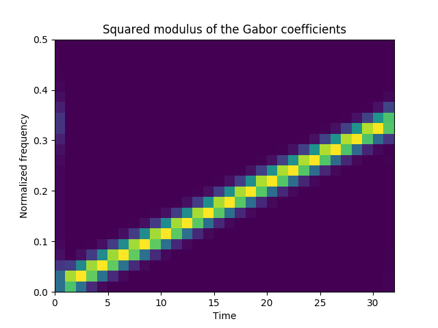
Gabor Representation of a Chirp with Oversampling

Figure 3.13 from the tutorial.

from tftb.generators import fmlin
from tftb.processing.linear import gabor
import matplotlib.pyplot as plt
import numpy as np

N1 = 256
Ng = 33
Q = 4
sig = fmlin(N1)[0]
window = np.exp(np.log(0.005) * np.linspace(-1, 1, Ng) ** 2)
window = window / np.linalg.norm(window)
tfr, dgr, h = gabor(sig, 32, Q, window)
time = np.arange(256)
freq = np.linspace(0, 0.5, 128)
plt.imshow(np.flipud(tfr)[8:, :], aspect='auto', extent=[0, 32, 0, 0.5],
           interpolation='none')
plt.xlabel('Time')
plt.ylabel('Normalized frequency')
plt.title('Squared modulus of the Gabor coefficients')
plt.show()