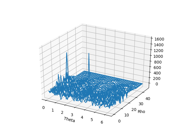
Hough-Wigner Transform of Two Simultaneous Chirps

Compute the Hough transform of the Wigner-Ville distribution of a signal composed of two chirps. Two peaks corresponding to the two chirps can be seen.

Figure 5.6 from the tutorial.

from tftb.generators import fmlin, sigmerge
from tftb.processing.cohen import WignerVilleDistribution
from tftb.processing.postprocessing import hough_transform
import numpy as np
from mpl_toolkits.mplot3d import Axes3D
import matplotlib.pyplot as plt

N = 64
sig = sigmerge(fmlin(N, 0, 0.4)[0], fmlin(N, 0.3, 0.5)[0], 1)
tfr, _, _ = WignerVilleDistribution(sig).run()

ht, rho, theta = hough_transform(tfr, N, N)
theta, rho = np.meshgrid(theta, rho)
fig = plt.figure()
ax = fig.gca(projection='3d')
ax.plot_wireframe(theta, rho, ht)
ax.set_xlabel('Theta')
ax.set_ylabel('Rho')
plt.show()