The spectrum \(X(\nu)\) is perfectly valid, but the Fourier transform is
essentially an integral over time. Thus, we lose all information that varies
with time. All we can tell from the spectrum is that the signal has two
distinct frequency components. In other words, we can comment on what happens
a signal, not when it happens. Consider a song as the signal under
consideration. If you were not interested in time, the whole point of
processing that signal would be lost. Rhythm and timing are the very heart of
good music, after all. In this case, we want to know when the drums kicked i
, as well as what notes were being played on the guitar. If we perform only
frequency analysis, all time information would be lost and the only
information we would have would be about what frequencies were played in the
song, and what their respective amplitudes were, averaged over the duration
of the entire song. So even if the drums stop playing after the second stanza,
the frequency spectrum would show them playing throughout the song.
Conversely, if we were only interested in the time information, we would be
hardly better off than simply listening to the song.
The solution to this problem is essentially time-frequency analysis which is
a field that deals with signal processing in both time and frequency domain.
It consists of a collection of methods that allow us to make tradeoffs
between time and frequency processing of a signal, depending on what makes
more sense for a particular application, as we shall see through the rest of
this tutorial.
Before delving into joint time frequency representations, it is necessary to
understand that any signal is characterized in the time-frequncy space by two
quantities:
The mean position of the signal, defined as pair of two figures: average
time (\(t_{m}\)) and average frequency (\(\nu_{m}\))
The energy localization of the signal in the time-frequency space, whose
area is proportional to the Time-Bandwidth product. An important
constraint related to this quantity is called the Heisenberg-Gabor
inequality, which we shall explore later in this section.
then the time and frequency domain energies of the signal can be considered as
probability distributions, and their respective means and standard deviations
can be used to estimate the time and frequency localizations and dispersions of
the signal.
Average time:
\(t_{m} = \frac{1}{E_{x}}\int_{-\infty}^{\infty}t\left|x(t)\right|^{2}dt\)
Average frequency:
\(\nu_{m} = \frac{1}{E_{x}}\int_{-\infty}^{\infty}\nu\left|X(\nu)\right|^{2}d\nu\)
Time spreading:
\(T^{2} = \frac{4\pi}{E_{x}}\int_{-\infty}^{\infty}(t-t_{m})^{2}\left|x(t)\right|^{2}dt\)
Frequency spreading:
\(B^{2} = \frac{4\pi}{E_{x}}\int_{-\infty}^{\infty}(\nu-\nu_{m})^{2}\left|X(\nu)\right|^{2}d\nu\)
Let’s play around with these values with some examples.
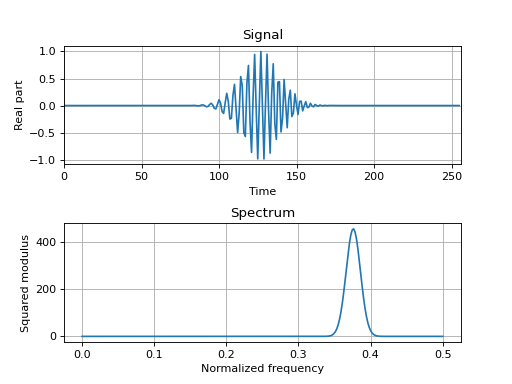
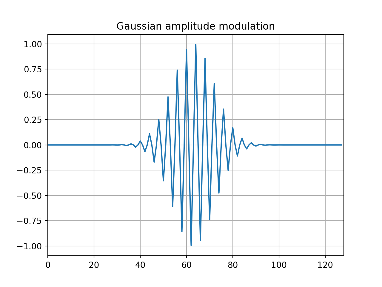
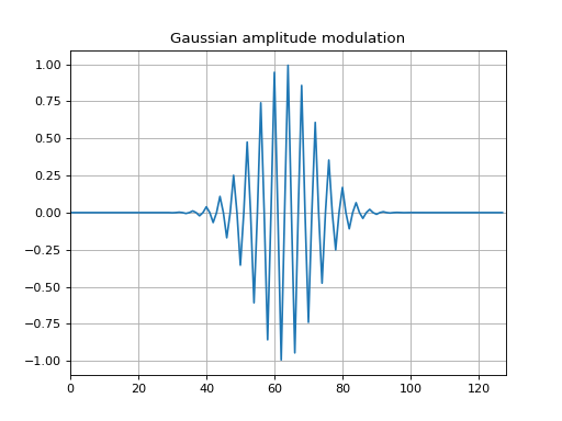
Time and frequency localizations can be calculated with the functions
tftb.processing.loctime and tftb.processing.locfreq. Consider a linear
chirp with Gaussian amplitude modulation as an example, shown below:
The time-bandwidth product of the signal can be obtained by multiplying the
time_spreading and frequency_spreading variables in the snippet above.
An important inequality concering the time bandwidth product is called the
uncertainty principle.
which states that a signal cannot be localized simultaneously in both time and
frequency with arbitrariy high resolution. The next example demonstrates this
concept.
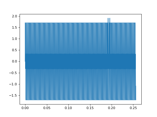
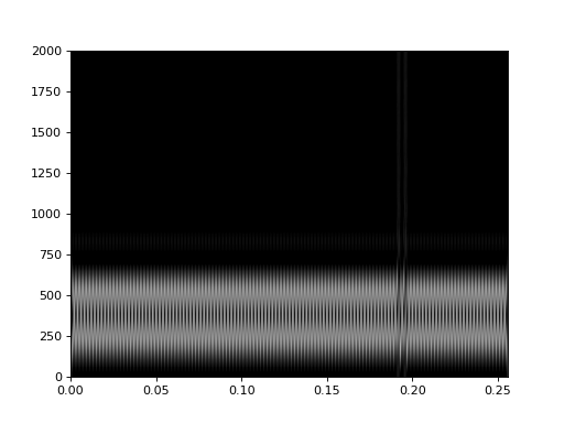
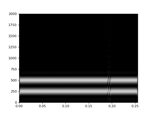
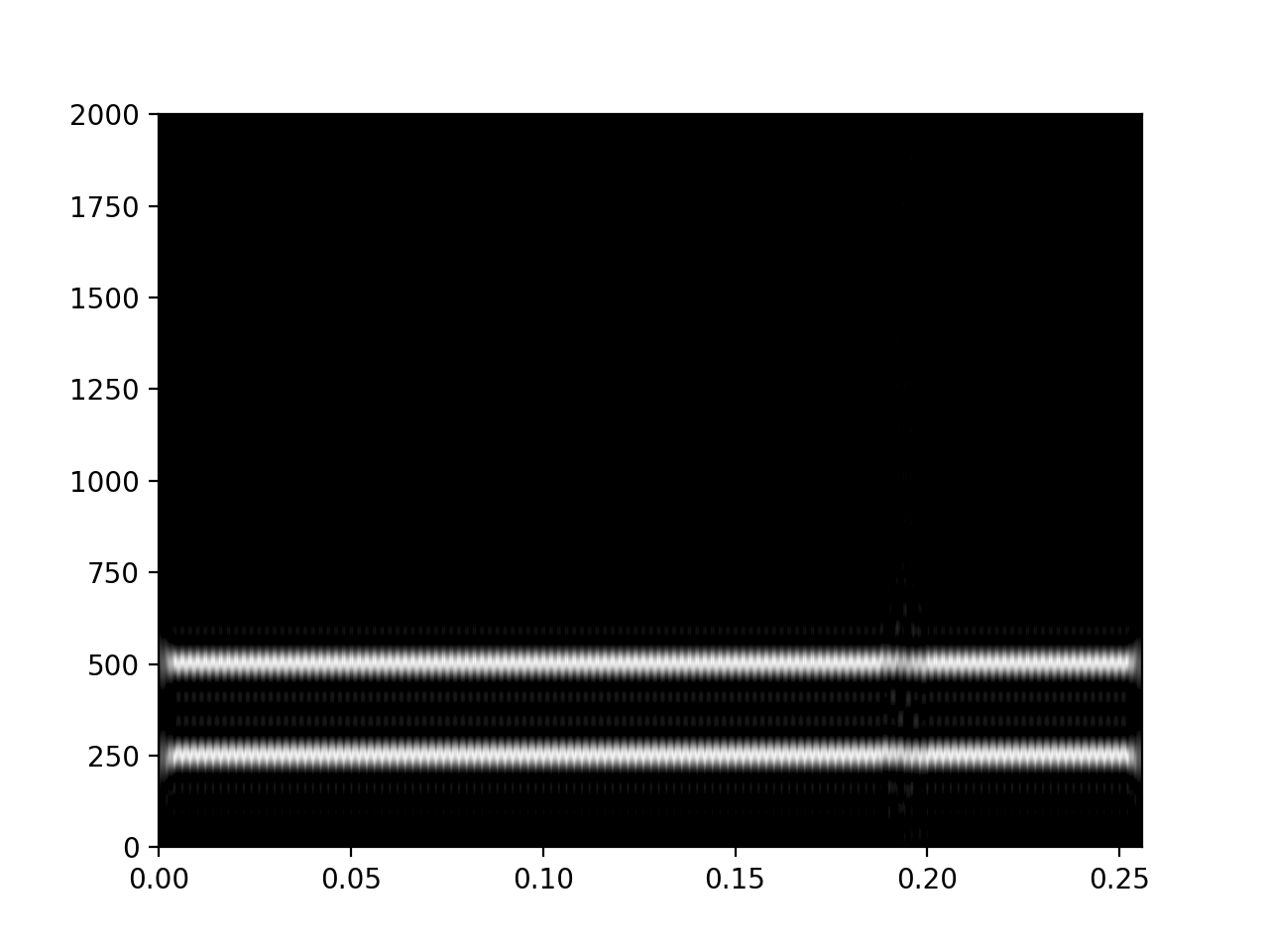
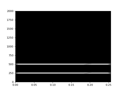
It is a sum of two sinusiodal signals of frequencies 500 Hz and 1000 Hz. It has
two spikes at \(t\) = 0.192s and \(t\) = 0.196s. The purpose of a time frequency
distribution would be to clearly identify both the frequencies and both the spikes,
thus resolving events in both frequency and time. Let’s check out the spectrograms of
of the signal with four different window lengths:
As can be clearly seen, resolution in time and frequency
cannot be obtained simultaneously. In the last (bottom) image, where the
window length is high, the STFT manages to discriminate between frequencies
of 500 Hz and 1000 Hz very clearly, but the time resolution between the
events at t = 0.192 s and t = 0.196 s is ambiguous. As we reduce the length
of the window function, the resolution between the time events goes on
becoming better, but only at the cost of resolution in frequencies.
Informally, the uncertainty principle states
that arbitrarily high resolution cannot be obtained in both time and frequency.
This is a consequence of the definition of the Fourier transform. The
definition insists that a signal be represented as a weighted sum of sinusoids,
and therefore identifies frequency information that is globally prevalent. As
a workaround to this interpretation, we use the STFT which performs the
Fourier transform on limited periods of the signals. Mathematically this
uncertainty can be quantified with the Heisenberg-Gabor Inequality (also
sometimes called the Gabor limit):
Heisenberg - Gabor Inequality
If \(T\) and \(B\) are standard deviations of the time
characteristics and the bandwidth respectively of a signal \(s(t)\),
then
\[TB ≥ 1\]
The expression states that the time-bandwidth product of a signal is lower
bounded by unity. Gaussian functions satisfy the equality condition in the
equation. This can be verified as follows:
A remarkably insightful commentary on the Uncertainty principle is provided
in 1, which states that the Uncertainty principle is a statement about two
variables whose associated operators do not mutually commute. This helps us
apply the Uncertainty principle in signal processing in the same way as in
quantum physics.
An alternative way to localize a signal in time and frequency is its
instantaneous frequency. Instantaneous frequencies are defined for analytic
signals, which are defined as follows
\[x_{a}(t) = x(t) + jH(x(t))\]
where \(x(t)\) is a real valued time domain signal and H denotes the
Hilbert transform (scipy.signal.hilbert). From this defition of the
analytic signal, the following quantities can be derived:
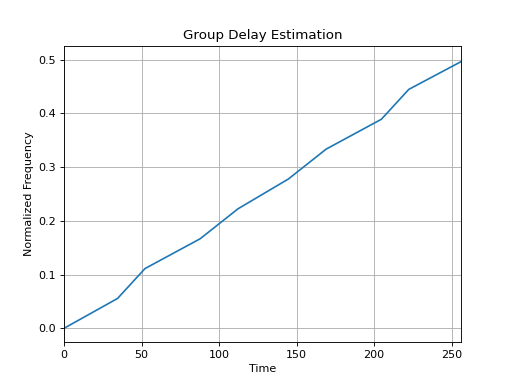
The frequency domain equivalent of instantaneous frequency is called group
delay, which localizes time characteristics of a signal as function of the
frequency.
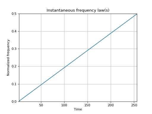
Example: Comparison of Instantaneous Frequency and Group Delay
Ideally, for a signal localized perfectly in time and frequency, its
instantaneous frequency and group delay would be expected to be identical.
However, mathematically they are two different fuctions in the time-frequency
space, and only coincide for signals with high time-bandwidth products. This
makes sense, since a high time-bandwidth product implies that the
signal would be pushed away from the Heisenberg-Gabor inequality, thereby
leading to lesser ambiguity. Consider the following example, where we construct
two signals - one with a high time-bandwidth product, and one with a low one -
and then estimate their respective instantaneous frequencies and group delays.
>>> # generate a signal with a high TB>>> time_instants=np.arange(2,256)>>> sig1=amgauss(256,128,90)*fmlin(256)[0]>>> tm,T1=loctime(sig1)>>> fm,B1=locfreq(sig1)>>> printT1*B115.9138>>> ifr1=inst_freq(sig1,time_instants)[0]>>> f1=np.linspace(0,0.5-1.0/256,256)>>> gd1=group_delay(sig1,f1)>>>>>> plt.subplot(211)>>> plt.plot(time_instants,ifr1,'*',label='inst_freq')>>> plt.plot(gd1,f1,'-',label='group delay')>>>>>> # generate a signal with low TB>>> sig2=amgauss(256,128,30)*fmlin(256,0.2,0.4)[0]>>> tm,T2=loctime(sig2)>>> fm,B2=locfreq(sig2)>>> printT2*B21.224>>> ifr2=inst_freq(sig2,time_instants)[0]>>> f2=np.linspace(0.02,0.4,256)>>> gd2=group_delay(sig2,f2)>>>>>> plt.subplot(212)>>> plt.plot(time_instants,ifr2,'*',label='inst_freq')>>> plt.plot(gd2,f2,'-',label='group delay')
As per Wikipedia, a “stationary” process is one whose joint probability
distribution does not change with time (or space). Let’s try and see what a
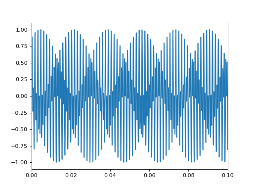
stationary process looks like. Consider a signal generated as follows:
The plot shows a slice of a touchtone signal with the duration of a tenth of a
second. This is the signal you hear when you press the “2” key on a telephone
dialing pad. (You can save the generated signal as a WAV file as follows:
and listen to the file tone.wav with your favourite music player.)
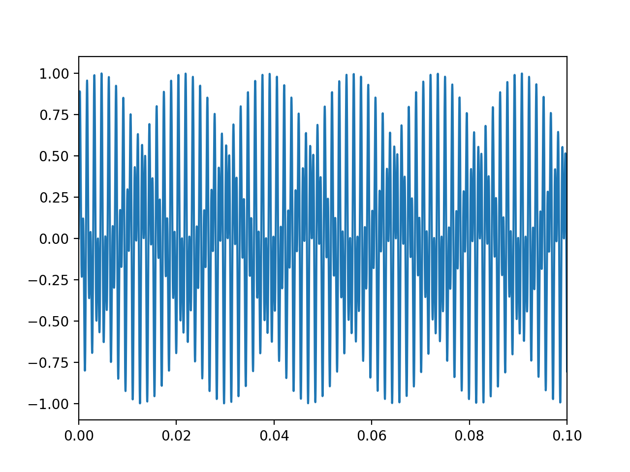
Since the signal is composed of two sinusoids, y1 and y2, we would
expect it to be stationary. Let’s try and assert this qualitatively. Let’s try
to plot the signal in its phase space. In order to do so, we will first need to
construct an analytic representation of the signal. For simplicity, we shall only
consider a part of the original signal
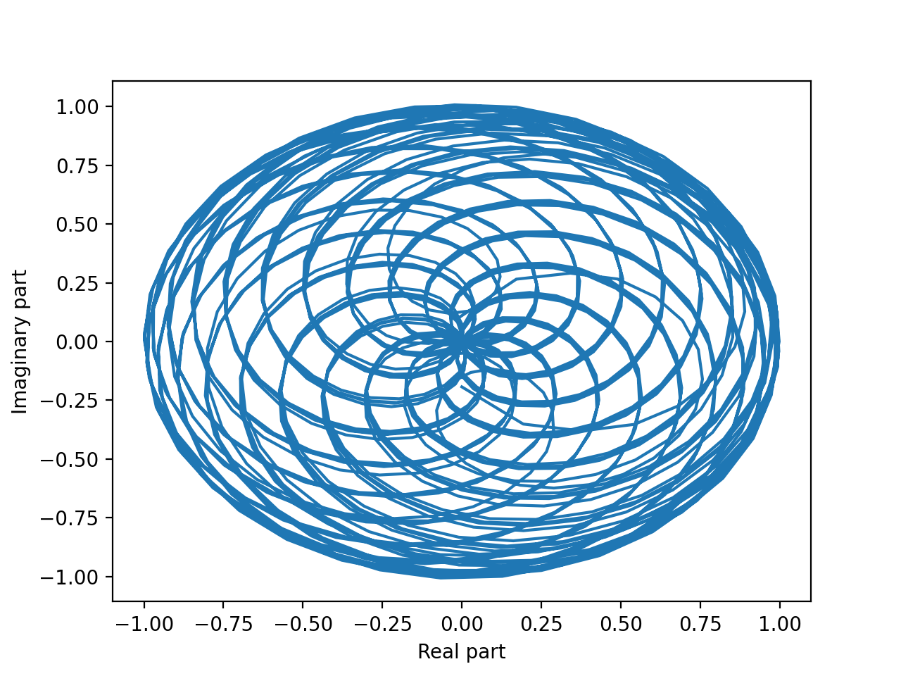
This visualization can be interpreted as follows. Imagine that there is a
vector centered at the origin of this plot which traces out the signal as it
rotates about the origin. Then, at any time \(t\), the angle which the
vector makes with the real axis is the instantaneous phase of the signal,
\(\theta(t)\). The angular speed with which the phasor rotates is the
instantaneous frequency of the signal:
\[\omega(t) = \frac{d}{dt} \theta(t)\]
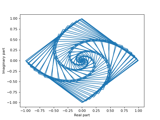
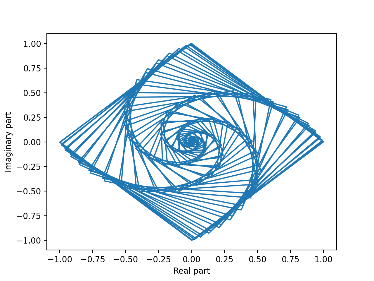
Now, let’s compare this phase plot with that of a known nonstationary signal.
>>> fromtftb.generatorsimportfmlin,amgauss>>> y_ns,_=fmlin(2048)# Already analytic, no need of Hilbert transorm>>> y_nonstat=y_ns*amgauss(2048)>>> plt.plot(np.real(y_nonstat),np.imag(y_nonstat))>>> plt.xlabel("Real part")>>> plt.ylabel("Imaginary part")>>> plt.show()
Notice that the second plot has a lot of rough edges and sharp angles. This
means that when the signal vector rotates through the phase space, it will have
to make sharp jumps in order to trace the signal. Moreover, by the definition
of instantaneous frequency, when the instantaneous phase is not differentiable,
the instantaneous frequency will be indeterminate. By contrast, the phase plot
for the stationary signal is a lot smoother, and we can expect that the
instantaneous frequency will be finite at all times. Physically, this means
that in the nonstationary signal, the variation in frequency components has no
structure, and these components can change arbitrarily.
This phenomenon of arbitrary, unstructured changes in frequency over time is a
symptom of nonstationarity, and will become increasingly relevant as we
proceed.
 >>> from tftb.generators import fmlin, amgauss >>> from tftb.processing import loctime, locfreq >>> sig = fmlin(256)[0] * amgauss(256) >>> t_mean, time_spreading = loctime(sig) >>> print t_mean, time_spreading 127.0 32.0 >>> f_mean, freq_spreading = locfreq(sig) >>> print f_mean, freq_spreading 0.249019607843 0.0700964323482


