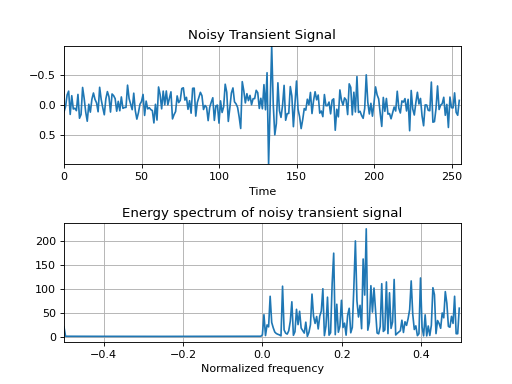
The second introductory example is a transient signal embedded in a -5 dB white gaussian noise. This transient signal
is a constant frequency modulated by a one-sided exponential amplitude. The signal and its spectrum are generated as
follows:
>>> importnumpyasnp>>> importmatplotlib.pyplotasplt>>> fromtftb.generatorsimportamexpos,fmconst,sigmerge,noisecg>>>>>> # Generate a noisy transient signal.>>> transsig=amexpos(64,kind='unilateral')*fmconst(64)[0]>>> signal=np.hstack((np.zeros((100,)),transsig,np.zeros((92,))))>>> signal=sigmerge(signal,noisecg(256),-5)>>> fig,ax=plt.subplots(2,1)>>> ax1,ax2=ax>>> ax1.plot(np.real(signal))>>> ax1.grid()>>> ax1.set_title('Noisy Transient Signal')>>> ax1.set_xlabel('Time')>>> ax1.set_xlim((0,256))>>> ax1.set_ylim((np.real(signal).max(),np.real(signal.min())))>>>>>> # Energy spectrum of the signal>>> dsp=np.fft.fftshift(np.abs(np.fft.fft(signal))**2)>>> ax2.plot(np.arange(-128,128,dtype=float)/256,dsp)>>> ax2.set_title('Energy spectrum of noisy transient signal')>>> ax2.set_xlabel('Normalized frequency')>>> ax2.grid()>>> ax2.set_xlim(-0.5,0.5)>>>>>> plt.subplots_adjust(hspace=0.5)>>>>>> plt.show()
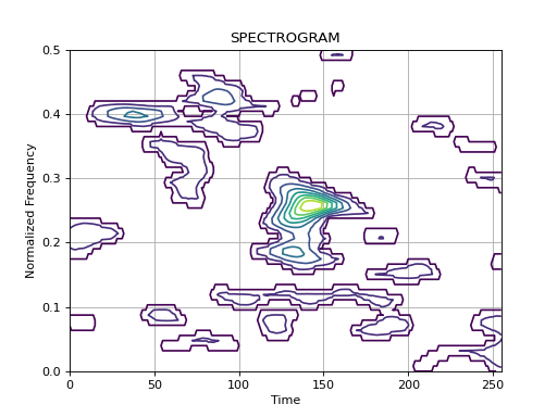
From these representations, it is difficult to localize precisely the signal in the time-domain as well as in the
frequency domain. Now let us have a look at the spectrogram of this signal: