tftb.processing package

Submodules

tftb.processing.affine module

Bilinear Time-Frequency Processing in the Affine Class.

class tftb.processing.affine.AffineDistribution(signal, fmin=None, fmax=None, **kwargs)

Bases: tftb.processing.base.BaseTFRepresentation

__init__(signal, fmin=None, fmax=None, **kwargs)

Create a base time-frequency representation object.

Parameters:

• signal (array-like) – Signal to be analyzed.
• **kwargs –

  Other arguments required for performing the analysis.

Returns:

BaseTFRepresentation object

Return type:

isaffine = True

plot(kind='contour', show_tf=True, threshold=0.05, **kwargs)

Visualize the time frequency representation.

Parameters:

• ax (matplotlib.axes.Axes object) – Axes object to draw the plot on.
• kind (str) – One of “cmap” (default), “contour”.
• show (bool) – Whether to call plt.show().
• default_annotation (bool) – Whether to make default annotations for the plot. Default annotations consist of setting the X and Y axis labels to “Time” and “Normalized Frequency” respectively, and setting the title to the name of the particular time-frequency distribution.
• show_tf – Whether to show the signal and it’s spectrum alongwith the plot. In this is True, the ax argument is ignored.
• **kwargs –

  Parameters to be passed to the plotting function.

Returns:

None

Return type:

None

run()

class tftb.processing.affine.BertrandDistribution(signal, fmin=None, fmax=None, n_voices=None, **kwargs)

Bases: tftb.processing.affine.AffineDistribution

__init__(signal, fmin=None, fmax=None, n_voices=None, **kwargs)

Create a base time-frequency representation object.

Parameters:

• signal (array-like) – Signal to be analyzed.
• **kwargs –

  Other arguments required for performing the analysis.

Returns:

BaseTFRepresentation object

Return type:

name = 'bertrand'

run()

class tftb.processing.affine.DFlandrinDistribution(signal, fmin=None, fmax=None, n_voices=None, **kwargs)

Bases: tftb.processing.affine.AffineDistribution

__init__(signal, fmin=None, fmax=None, n_voices=None, **kwargs)

Create a base time-frequency representation object.

Parameters:

• signal (array-like) – Signal to be analyzed.
• **kwargs –

  Other arguments required for performing the analysis.

Returns:

BaseTFRepresentation object

Return type:

name = 'd-flandrin'

run()

class tftb.processing.affine.Scalogram(signal, fmin=None, fmax=None, n_voices=None, waveparams=None, **kwargs)

Bases: tftb.processing.affine.AffineDistribution

Morlet Scalogram.

__init__(signal, fmin=None, fmax=None, n_voices=None, waveparams=None, **kwargs)

Create a base time-frequency representation object.

Parameters:

• signal (array-like) – Signal to be analyzed.
• **kwargs –

  Other arguments required for performing the analysis.

Returns:

BaseTFRepresentation object

Return type:

isaffine = False

name = 'scalogram'

run()

class tftb.processing.affine.UnterbergerDistribution(signal, form='A', fmin=None, fmax=None, n_voices=None, **kwargs)

Bases: tftb.processing.affine.AffineDistribution

__init__(signal, form='A', fmin=None, fmax=None, n_voices=None, **kwargs)

Create a base time-frequency representation object.

Parameters:

• signal (array-like) – Signal to be analyzed.
• **kwargs –

  Other arguments required for performing the analysis.

Returns:

BaseTFRepresentation object

Return type:

name = 'unterberger'

run()

tftb.processing.affine.lambdak(u, k)

tftb.processing.affine.smoothed_pseudo_wigner(signal, timestamps=None, K='bertrand', nh0=None, ng0=0, fmin=None, fmax=None, n_voices=None)

Parameters:

• signal –
• timestamps –
• K –
• nh0 –
• ng0 –
• fmin –
• fmax –
• n_voices –

Returns:

Return type:

tftb.processing.affine.umaxdfla_solve(ratio)

tftb.processing.ambiguity module

Ambiguity functions.

tftb.processing.ambiguity.narrow_band(signal, lag=None, n_fbins=None)

Narrow band ambiguity function.

Parameters:

• signal (array-like) – Signal to be analyzed.
• lag (array-like) – vector of lag values.
• n_fbins (int) – number of frequency bins

Returns:

Doppler lag representation

Return type:

array-like

tftb.processing.ambiguity.wide_band(signal, fmin=None, fmax=None, N=None)

tftb.processing.base module

Base time-frequency representation class.

class tftb.processing.base.BaseTFRepresentation(signal, **kwargs)

Bases: object

__init__(signal, **kwargs)

Create a base time-frequency representation object.

Parameters:

• signal (array-like) – Signal to be analyzed.
• **kwargs –

  Other arguments required for performing the analysis.

Returns:

BaseTFRepresentation object

Return type:

isaffine = False

plot(ax=None, kind='cmap', show=True, default_annotation=True, show_tf=False, scale='linear', threshold=0.05, **kwargs)

Visualize the time frequency representation.

Parameters:

• ax (matplotlib.axes.Axes object) – Axes object to draw the plot on.
• kind (str) – One of “cmap” (default), “contour”.
• show (bool) – Whether to call plt.show().
• default_annotation (bool) – Whether to make default annotations for the plot. Default annotations consist of setting the X and Y axis labels to “Time” and “Normalized Frequency” respectively, and setting the title to the name of the particular time-frequency distribution.
• show_tf – Whether to show the signal and it’s spectrum alongwith the plot. In this is True, the ax argument is ignored.
• **kwargs –

  Parameters to be passed to the plotting function.

Returns:

None

Return type:

None

tftb.processing.cohen module

Bilinear Time-Frequency Processing in the Cohen’s Class.

class tftb.processing.cohen.MargenauHillDistribution(signal, **kwargs)

Bases: tftb.processing.base.BaseTFRepresentation

name = 'margenau-hill'

plot(kind='cmap', threshold=0.05, sqmod=True, **kwargs)

Visualize the time frequency representation.

Parameters:

• ax (matplotlib.axes.Axes object) – Axes object to draw the plot on.
• kind (str) – One of “cmap” (default), “contour”.
• show (bool) – Whether to call plt.show().
• default_annotation (bool) – Whether to make default annotations for the plot. Default annotations consist of setting the X and Y axis labels to “Time” and “Normalized Frequency” respectively, and setting the title to the name of the particular time-frequency distribution.
• show_tf – Whether to show the signal and it’s spectrum alongwith the plot. In this is True, the ax argument is ignored.
• **kwargs –

  Parameters to be passed to the plotting function.

Returns:

None

Return type:

None

run()

class tftb.processing.cohen.PageRepresentation(signal, **kwargs)

Bases: tftb.processing.base.BaseTFRepresentation

name = 'page representation'

plot(kind='cmap', threshold=0.05, sqmod=True, **kwargs)

Visualize the time frequency representation.

Parameters:

• ax (matplotlib.axes.Axes object) – Axes object to draw the plot on.
• kind (str) – One of “cmap” (default), “contour”.
• show (bool) – Whether to call plt.show().
• default_annotation (bool) – Whether to make default annotations for the plot. Default annotations consist of setting the X and Y axis labels to “Time” and “Normalized Frequency” respectively, and setting the title to the name of the particular time-frequency distribution.
• show_tf – Whether to show the signal and it’s spectrum alongwith the plot. In this is True, the ax argument is ignored.
• **kwargs –

  Parameters to be passed to the plotting function.

Returns:

None

Return type:

None

run()

class tftb.processing.cohen.PseudoMargenauHillDistribution(signal, **kwargs)

Bases: tftb.processing.cohen.MargenauHillDistribution

name = 'pseudo margenau-hill'

run()

class tftb.processing.cohen.PseudoPageRepresentation(signal, **kwargs)

Bases: tftb.processing.cohen.PageRepresentation

name = 'pseudo page'

run()

class tftb.processing.cohen.PseudoWignerVilleDistribution(signal, **kwargs)

Bases: tftb.processing.cohen.WignerVilleDistribution

name = 'pseudo winger-ville'

plot(**kwargs)

Visualize the time frequency representation.

Parameters:

• ax (matplotlib.axes.Axes object) – Axes object to draw the plot on.
• kind (str) – One of “cmap” (default), “contour”.
• show (bool) – Whether to call plt.show().
• default_annotation (bool) – Whether to make default annotations for the plot. Default annotations consist of setting the X and Y axis labels to “Time” and “Normalized Frequency” respectively, and setting the title to the name of the particular time-frequency distribution.
• show_tf – Whether to show the signal and it’s spectrum alongwith the plot. In this is True, the ax argument is ignored.
• **kwargs –

  Parameters to be passed to the plotting function.

Returns:

None

Return type:

None

run()

class tftb.processing.cohen.Spectrogram(signal, timestamps=None, n_fbins=None, fwindow=None)

Bases: tftb.processing.linear.ShortTimeFourierTransform

name = 'spectrogram'

plot(kind='cmap', **kwargs)

Display the spectrogram of an STFT.

Parameters:

• ax (matplotlib.axes.Axes object) – axes object to draw the plot on. If None(default), one will be created.
• kind (str) – Choice of visualization type, either “cmap”(default) or “contour”.
• sqmod (bool) – Whether to take squared modulus of TFR before plotting. (Default: True)
• threshold (float) – Percentage of the maximum value of the TFR, below which all values are set to zero before plotting.
• **kwargs –

  parameters passed to the plotting function.

Returns:

None

Return type:

None

run()

Compute the STFT according to:

\[X[m, w] = \sum_{n=-\infty}^{\infty}x[n]w[n - m]e^{-j\omega n}\]

Where \(w\) is a Hamming window.

class tftb.processing.cohen.WignerVilleDistribution(signal, **kwargs)

Bases: tftb.processing.base.BaseTFRepresentation

name = 'wigner-ville'

plot(kind='cmap', threshold=0.05, sqmod=False, **kwargs)

Visualize the time frequency representation.

Parameters:

• ax (matplotlib.axes.Axes object) – Axes object to draw the plot on.
• kind (str) – One of “cmap” (default), “contour”.
• show (bool) – Whether to call plt.show().
• default_annotation (bool) – Whether to make default annotations for the plot. Default annotations consist of setting the X and Y axis labels to “Time” and “Normalized Frequency” respectively, and setting the title to the name of the particular time-frequency distribution.
• show_tf – Whether to show the signal and it’s spectrum alongwith the plot. In this is True, the ax argument is ignored.
• **kwargs –

  Parameters to be passed to the plotting function.

Returns:

None

Return type:

None

run()

tftb.processing.cohen.smoothed_pseudo_wigner_ville(signal, timestamps=None, freq_bins=None, twindow=None, fwindow=None)

Smoothed Pseudo Wigner-Ville time-frequency distribution. :param signal: signal to be analyzed :param timestamps: time instants of the signal :param freq_bins: number of frequency bins :param twindow: time smoothing window :param fwindow: frequency smoothing window :type signal: array-like :type timestamps: array-like :type freq_bins: int :type twindow: array-like :type fwindow: array-like :return: Smoothed pseudo Wigner Ville distribution :rtype: array-like

tftb.processing.freq_domain module

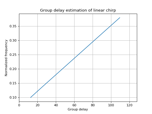
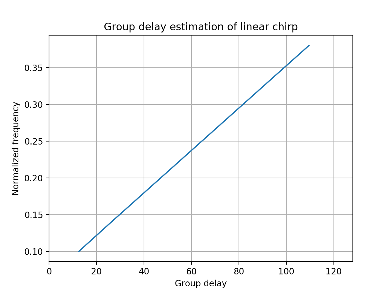
tftb.processing.freq_domain.group_delay(x, fnorm=None)

Compute the group delay of a signal at normalized frequencies.

Parameters:

• x (numpy.ndarray) – time domain signal
• fnorm (float) – normalized frequency at which to calculate the group delay.

Returns:

group delay

Return type:

numpy.ndarray

Example:

>>> import numpy as np
>>> from tftb.generators import amgauss, fmlin
>>> x = amgauss(128, 64.0, 30) * fmlin(128, 0.1, 0.4)[0]
>>> fnorm = np.arange(0.1, 0.38, step=0.04)
>>> gd = group_delay(x, fnorm)
>>> plot(gd, fnorm) #doctest: +SKIP

(Source code, png, hires.png, pdf)

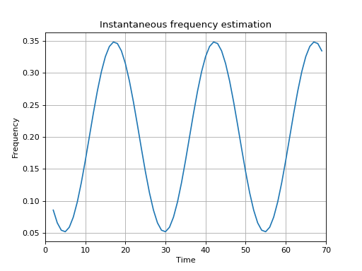
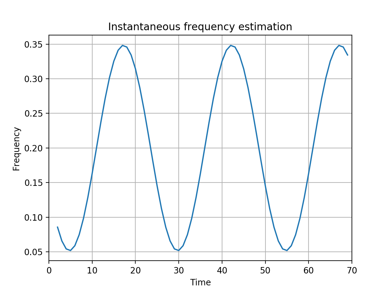
tftb.processing.freq_domain.inst_freq(x, t=None, L=1)

Compute the instantaneous frequency of an analytic signal at specific time instants using the trapezoidal integration rule.

Parameters:

• x (numpy.ndarray) – The input analytic signal
• t (numpy.ndarray) – The time instants at which to calculate the instantaneous frequencies.
• L (int) – Non default values are currently not supported. If L is 1, the normalized instantaneous frequency is computed. If L > 1, the maximum likelihood estimate of the instantaneous frequency of the deterministic part of the signal.

Returns:

instantaneous frequencies of the input signal.

Return type:

numpy.ndarray

Example:

>>> from tftb.generators import fmsin
>>> x = fmsin(70, 0.05, 0.35, 25)[0]
>>> instf, timestamps = inst_freq(x)
>>> plot(timestamps, instf) #doctest: +SKIP

(Source code, png, hires.png, pdf)

tftb.processing.freq_domain.locfreq(signal)

Compute the frequency localization characteristics.

Parameters:sig (numpy.ndarray) – input signal Returns:average normalized frequency center, frequency spreading Return type:tuple Example:

>>> from tftb.generators import amgauss
>>> z = amgauss(160, 80, 50)
>>> fm, B = locfreq(z)
>>> print("%.3g" % fm)
-9.18e-14
>>> print("%.4g" % B)
0.02

tftb.processing.linear module

Linear Time Frequency Processing.

class tftb.processing.linear.ShortTimeFourierTransform(signal, timestamps=None, n_fbins=None, fwindow=None)

Bases: tftb.processing.base.BaseTFRepresentation

Short time Fourier transform.

__init__(signal, timestamps=None, n_fbins=None, fwindow=None)

Create a ShortTimeFourierTransform object.

Parameters:

• signal (array-like) – Signal to be analyzed.
• timestamps (array-like) – Time instants of the signal (default: np.arange(len(signal)))
• n_fbins (int) – Number of frequency bins (default: len(signal))
• fwindow (array-like) – Frequency smoothing window (default: Hamming window of length len(signal) / 4)

Returns:

ShortTimeFourierTransform object

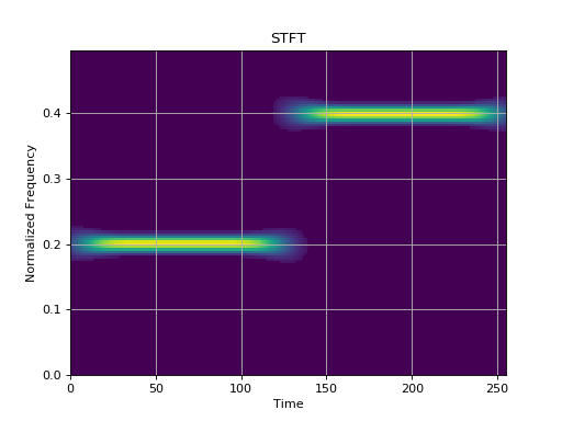
Example:

>>> from tftb.generators import fmconst
>>> sig = np.r_[fmconst(128, 0.2)[0], fmconst(128, 0.4)[0]]
>>> stft = ShortTimeFourierTransform(sig)
>>> tfr, t, f = stft.run()
>>> stft.plot() #doctest: +SKIP

(Source code, png, hires.png, pdf)

name = 'stft'

plot(ax=None, kind='cmap', sqmod=True, threshold=0.05, **kwargs)

Display the spectrogram of an STFT.

Parameters:

• ax (matplotlib.axes.Axes object) – axes object to draw the plot on. If None(default), one will be created.
• kind (str) – Choice of visualization type, either “cmap”(default) or “contour”.
• sqmod (bool) – Whether to take squared modulus of TFR before plotting. (Default: True)
• threshold (float) – Percentage of the maximum value of the TFR, below which all values are set to zero before plotting.
• **kwargs –

  parameters passed to the plotting function.

Returns:

None

Return type:

None

run()

Compute the STFT according to:

\[X[m, w] = \sum_{n=-\infty}^{\infty}x[n]w[n - m]e^{-j\omega n}\]

Where \(w\) is a Hamming window.

tftb.processing.linear.gabor(signal, n_coeff=None, q_oversample=None, window=None)

Compute the Gabor representation of a signal.

Parameters:

• signal (array-like) – Singal to be analyzed.
• n_coeff (integer) – number of Gabor coefficients in time.
• q_oversample (int) – Degree of oversampling
• window (array-like) – Synthesis window

Returns:

Tuple of Gabor coefficients, biorthogonal window associated with the synthesis window.

Return type:

tuple

tftb.processing.plotifl module

tftb.processing.plotifl.plotifl(time_instants, iflaws, signal=None, **kwargs)

Plot normalized instantaneous frequency laws.

Parameters:

• time_instants (array-like) – timestamps of the signal
• iflaws (array-like) – instantaneous freqency law(s) of the signal.
• signal (array-like) – if provided, display it.

Returns:

None

tftb.processing.postprocessing module

Postprocessing functions.

tftb.processing.postprocessing.friedman_density(tfr, re_mat, timestamps=None)

Parameters:

• tfr –
• re_mat –
• timestamps –

Returns:

Return type:

tftb.processing.postprocessing.hough_transform(image, m=None, n=None)

Parameters:

• image –
• m –
• n –

Returns:

Return type:

tftb.processing.postprocessing.ideal_tfr(iflaws, timestamps=None, n_fbins=None)

Parameters:

• iflaws –
• timestamps –
• n_fbins –

Returns:

Return type:

tftb.processing.postprocessing.renyi_information(tfr, timestamps=None, freq=None, alpha=3.0)

Parameters:

• tfr –
• timestamps –
• freq –
• alpha –

Returns:

Return type:

tftb.processing.postprocessing.ridges(tfr, re_mat, timestamps=None, method='rsp')

Parameters:

• tfr –
• re_mat –
• timestamps –
• method –

Returns:

Return type:

tftb.processing.reassigned module

Reassigned TF processing.

tftb.processing.reassigned.morlet_scalogram(signal, timestamps=None, n_fbins=None, tbp=0.25)

param signal: param timestamps:   param n_fbins: param tbp: type signal: type timestamps:   type n_fbins: type tbp:

Returns: Return type:

tftb.processing.reassigned.pseudo_margenau_hill(signal, timestamps=None, n_fbins=None, fwindow=None)

param signal: param timestamps:   param n_fbins: param fwindow: type signal: type timestamps:   type n_fbins: type fwindow:

Returns: Return type:

tftb.processing.reassigned.pseudo_page(signal, timestamps=None, n_fbins=None, fwindow=None)

param signal: param timestamps:   param n_fbins: param fwindow: type signal: type timestamps:   type n_fbins: type fwindow:

Returns: Return type:

tftb.processing.reassigned.pseudo_wigner_ville(signal, timestamps=None, n_fbins=None, fwindow=None)

param signal: param timestamps:   param n_fbins: param fwindow: type signal: type timestamps:   type n_fbins: type fwindow:

Returns: Return type:

tftb.processing.reassigned.smoothed_pseudo_wigner_ville(signal, timestamps=None, n_fbins=None, twindow=None, fwindow=None)

param signal: param timestamps:   param n_fbins: param twindow: param fwindow: type signal: type timestamps:   type n_fbins: type twindow: type fwindow:

Returns: Return type:

tftb.processing.reassigned.spectrogram(signal, time_samples=None, n_fbins=None, window=None)

Compute the spectrogram and reassigned spectrogram.

Parameters:

• signal (array-like) – signal to be analzsed
• time_samples (array-like) – time instants (default: np.arange(len(signal)))
• n_fbins (int) – number of frequency bins (default: len(signal))
• window (array-like) – frequency smoothing window (default: Hamming with size=len(signal)/4)

Returns:

spectrogram, reassigned specstrogram and matrix of reassignment

vectors :rtype: tuple(array-like)

tftb.processing.time_domain module

tftb.processing.time_domain.loctime(sig)

Compute the time localization characteristics.

Parameters:sig (numpy.ndarray) – input signal Returns:Average time center and time spreading Return type:tuple Example:

>>> from tftb.generators import amgauss
>>> x = amgauss(160, 80.0, 50.0)
>>> tm, T = loctime(x)
>>> print("%.2f" % tm)
79.00
>>> print("%.2f" % T)
50.00

tftb.processing.utils module

Miscellaneous processing utilities.

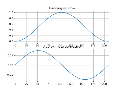
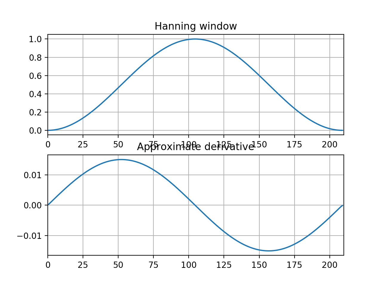
tftb.processing.utils.derive_window(window)

Calculate derivative of a window function.

Parameters:window – Window function to be differentiated. This is expected to be

a standard window function with an odd length. :type window: array-like :return: Derivative of the input window :rtype: array-like :Example: >>> from scipy.signal import hanning >>> import matplotlib.pyplot as plt #doctest: +SKIP >>> window = hanning(210) >>> derivation = derive_window(window) >>> plt.subplot(211), plt.plot(window) #doctest: +SKIP >>> plt.subplot(212), plt.plot(derivation) #doctest: +SKIP

(Source code, png, hires.png, pdf)

tftb.processing.utils.get_spectrum(signal)

tftb.processing.utils.integrate_2d(mat, x=None, y=None)

param mat: param x: param y: type mat: type x: type y:

Returns: Return type:

Example:

>>> from __future__ import print_function
>>> from tftb.generators import altes
>>> from tftb.processing import Scalogram
>>> x = altes(256, 0.1, 0.45, 10000)
>>> tfr, t, f, _ = Scalogram(x).run()
>>> print("%.3f" % integrate_2d(tfr, t, f))
2.000

Module contents

tftb.processing.loctime(sig)

Compute the time localization characteristics.

Parameters:sig (numpy.ndarray) – input signal Returns:Average time center and time spreading Return type:tuple Example:

>>> from tftb.generators import amgauss
>>> x = amgauss(160, 80.0, 50.0)
>>> tm, T = loctime(x)
>>> print("%.2f" % tm)
79.00
>>> print("%.2f" % T)
50.00

tftb.processing.locfreq(signal)

Compute the frequency localization characteristics.

Parameters:sig (numpy.ndarray) – input signal Returns:average normalized frequency center, frequency spreading Return type:tuple Example:

>>> from tftb.generators import amgauss
>>> z = amgauss(160, 80, 50)
>>> fm, B = locfreq(z)
>>> print("%.3g" % fm)
-9.18e-14
>>> print("%.4g" % B)
0.02

tftb.processing.inst_freq(x, t=None, L=1)

Compute the instantaneous frequency of an analytic signal at specific time instants using the trapezoidal integration rule.

Parameters:

• x (numpy.ndarray) – The input analytic signal
• t (numpy.ndarray) – The time instants at which to calculate the instantaneous frequencies.
• L (int) – Non default values are currently not supported. If L is 1, the normalized instantaneous frequency is computed. If L > 1, the maximum likelihood estimate of the instantaneous frequency of the deterministic part of the signal.

Returns:

instantaneous frequencies of the input signal.

Return type:

numpy.ndarray

Example:

>>> from tftb.generators import fmsin
>>> x = fmsin(70, 0.05, 0.35, 25)[0]
>>> instf, timestamps = inst_freq(x)
>>> plot(timestamps, instf) #doctest: +SKIP

(Source code, png, hires.png, pdf)

tftb.processing.group_delay(x, fnorm=None)

Compute the group delay of a signal at normalized frequencies.

Parameters:

• x (numpy.ndarray) – time domain signal
• fnorm (float) – normalized frequency at which to calculate the group delay.

Returns:

group delay

Return type:

numpy.ndarray

Example:

>>> import numpy as np
>>> from tftb.generators import amgauss, fmlin
>>> x = amgauss(128, 64.0, 30) * fmlin(128, 0.1, 0.4)[0]
>>> fnorm = np.arange(0.1, 0.38, step=0.04)
>>> gd = group_delay(x, fnorm)
>>> plot(gd, fnorm) #doctest: +SKIP

(Source code, png, hires.png, pdf)

tftb.processing.plotifl(time_instants, iflaws, signal=None, **kwargs)

Plot normalized instantaneous frequency laws.

Parameters:

• time_instants (array-like) – timestamps of the signal
• iflaws (array-like) – instantaneous freqency law(s) of the signal.
• signal (array-like) – if provided, display it.

Returns:

None

class tftb.processing.WignerVilleDistribution(signal, **kwargs)

Bases: tftb.processing.base.BaseTFRepresentation

name = 'wigner-ville'

plot(kind='cmap', threshold=0.05, sqmod=False, **kwargs)

Visualize the time frequency representation.

Parameters:

• ax (matplotlib.axes.Axes object) – Axes object to draw the plot on.
• kind (str) – One of “cmap” (default), “contour”.
• show (bool) – Whether to call plt.show().
• default_annotation (bool) – Whether to make default annotations for the plot. Default annotations consist of setting the X and Y axis labels to “Time” and “Normalized Frequency” respectively, and setting the title to the name of the particular time-frequency distribution.
• show_tf – Whether to show the signal and it’s spectrum alongwith the plot. In this is True, the ax argument is ignored.
• **kwargs –

  Parameters to be passed to the plotting function.

Returns:

None

Return type:

None

run()

class tftb.processing.PseudoWignerVilleDistribution(signal, **kwargs)

Bases: tftb.processing.cohen.WignerVilleDistribution

name = 'pseudo winger-ville'

plot(**kwargs)

Visualize the time frequency representation.

Parameters:

• ax (matplotlib.axes.Axes object) – Axes object to draw the plot on.
• kind (str) – One of “cmap” (default), “contour”.
• show (bool) – Whether to call plt.show().
• default_annotation (bool) – Whether to make default annotations for the plot. Default annotations consist of setting the X and Y axis labels to “Time” and “Normalized Frequency” respectively, and setting the title to the name of the particular time-frequency distribution.
• show_tf – Whether to show the signal and it’s spectrum alongwith the plot. In this is True, the ax argument is ignored.
• **kwargs –

  Parameters to be passed to the plotting function.

Returns:

None

Return type:

None

run()

tftb.processing.smoothed_pseudo_wigner_ville(signal, timestamps=None, freq_bins=None, twindow=None, fwindow=None)

Smoothed Pseudo Wigner-Ville time-frequency distribution. :param signal: signal to be analyzed :param timestamps: time instants of the signal :param freq_bins: number of frequency bins :param twindow: time smoothing window :param fwindow: frequency smoothing window :type signal: array-like :type timestamps: array-like :type freq_bins: int :type twindow: array-like :type fwindow: array-like :return: Smoothed pseudo Wigner Ville distribution :rtype: array-like

class tftb.processing.MargenauHillDistribution(signal, **kwargs)

Bases: tftb.processing.base.BaseTFRepresentation

name = 'margenau-hill'

plot(kind='cmap', threshold=0.05, sqmod=True, **kwargs)

Visualize the time frequency representation.

Parameters:

• ax (matplotlib.axes.Axes object) – Axes object to draw the plot on.
• kind (str) – One of “cmap” (default), “contour”.
• show (bool) – Whether to call plt.show().
• default_annotation (bool) – Whether to make default annotations for the plot. Default annotations consist of setting the X and Y axis labels to “Time” and “Normalized Frequency” respectively, and setting the title to the name of the particular time-frequency distribution.
• show_tf – Whether to show the signal and it’s spectrum alongwith the plot. In this is True, the ax argument is ignored.
• **kwargs –

  Parameters to be passed to the plotting function.

Returns:

None

Return type:

None

run()

class tftb.processing.Spectrogram(signal, timestamps=None, n_fbins=None, fwindow=None)

Bases: tftb.processing.linear.ShortTimeFourierTransform

name = 'spectrogram'

plot(kind='cmap', **kwargs)

Display the spectrogram of an STFT.

Parameters:

• ax (matplotlib.axes.Axes object) – axes object to draw the plot on. If None(default), one will be created.
• kind (str) – Choice of visualization type, either “cmap”(default) or “contour”.
• sqmod (bool) – Whether to take squared modulus of TFR before plotting. (Default: True)
• threshold (float) – Percentage of the maximum value of the TFR, below which all values are set to zero before plotting.
• **kwargs –

  parameters passed to the plotting function.

Returns:

None

Return type:

None

run()

Compute the STFT according to:

\[X[m, w] = \sum_{n=-\infty}^{\infty}x[n]w[n - m]e^{-j\omega n}\]

Where \(w\) is a Hamming window.

tftb.processing.reassigned_spectrogram(signal, time_samples=None, n_fbins=None, window=None)

Compute the spectrogram and reassigned spectrogram.

Parameters:

• signal (array-like) – signal to be analzsed
• time_samples (array-like) – time instants (default: np.arange(len(signal)))
• n_fbins (int) – number of frequency bins (default: len(signal))
• window (array-like) – frequency smoothing window (default: Hamming with size=len(signal)/4)

Returns:

spectrogram, reassigned specstrogram and matrix of reassignment

vectors :rtype: tuple(array-like)

tftb.processing.reassigned_smoothed_pseudo_wigner_ville(signal, timestamps=None, n_fbins=None, twindow=None, fwindow=None)

smoothed_pseudo_wigner_ville

param signal: param timestamps:   param n_fbins: param twindow: param fwindow: type signal: type timestamps:   type n_fbins: type twindow: type fwindow:

Returns: Return type:

tftb.processing.ideal_tfr(iflaws, timestamps=None, n_fbins=None)

Parameters:

• iflaws –
• timestamps –
• n_fbins –

Returns:

Return type:

tftb.processing.renyi_information(tfr, timestamps=None, freq=None, alpha=3.0)

Parameters:

• tfr –
• timestamps –
• freq –
• alpha –

Returns:

Return type:

class tftb.processing.Scalogram(signal, fmin=None, fmax=None, n_voices=None, waveparams=None, **kwargs)

Bases: tftb.processing.affine.AffineDistribution

Morlet Scalogram.

__init__(signal, fmin=None, fmax=None, n_voices=None, waveparams=None, **kwargs)

Create a base time-frequency representation object.

Parameters:

• signal (array-like) – Signal to be analyzed.
• **kwargs –

  Other arguments required for performing the analysis.

Returns:

BaseTFRepresentation object

Return type:

isaffine = False

name = 'scalogram'

run()

class tftb.processing.BertrandDistribution(signal, fmin=None, fmax=None, n_voices=None, **kwargs)

Bases: tftb.processing.affine.AffineDistribution

__init__(signal, fmin=None, fmax=None, n_voices=None, **kwargs)

Create a base time-frequency representation object.

Parameters:

• signal (array-like) – Signal to be analyzed.
• **kwargs –

  Other arguments required for performing the analysis.

Returns:

BaseTFRepresentation object

Return type:

name = 'bertrand'

run()

class tftb.processing.DFlandrinDistribution(signal, fmin=None, fmax=None, n_voices=None, **kwargs)

Bases: tftb.processing.affine.AffineDistribution

__init__(signal, fmin=None, fmax=None, n_voices=None, **kwargs)

Create a base time-frequency representation object.

Parameters:

• signal (array-like) – Signal to be analyzed.
• **kwargs –

  Other arguments required for performing the analysis.

Returns:

BaseTFRepresentation object

Return type:

name = 'd-flandrin'

run()

class tftb.processing.UnterbergerDistribution(signal, form='A', fmin=None, fmax=None, n_voices=None, **kwargs)

Bases: tftb.processing.affine.AffineDistribution

__init__(signal, form='A', fmin=None, fmax=None, n_voices=None, **kwargs)

Create a base time-frequency representation object.

Parameters:

• signal (array-like) – Signal to be analyzed.
• **kwargs –

  Other arguments required for performing the analysis.

Returns:

BaseTFRepresentation object

Return type:

name = 'unterberger'

run()

class tftb.processing.ShortTimeFourierTransform(signal, timestamps=None, n_fbins=None, fwindow=None)

Bases: tftb.processing.base.BaseTFRepresentation

Short time Fourier transform.

__init__(signal, timestamps=None, n_fbins=None, fwindow=None)

Create a ShortTimeFourierTransform object.

Parameters:

• signal (array-like) – Signal to be analyzed.
• timestamps (array-like) – Time instants of the signal (default: np.arange(len(signal)))
• n_fbins (int) – Number of frequency bins (default: len(signal))
• fwindow (array-like) – Frequency smoothing window (default: Hamming window of length len(signal) / 4)

Returns:

ShortTimeFourierTransform object

Example:

>>> from tftb.generators import fmconst
>>> sig = np.r_[fmconst(128, 0.2)[0], fmconst(128, 0.4)[0]]
>>> stft = ShortTimeFourierTransform(sig)
>>> tfr, t, f = stft.run()
>>> stft.plot() #doctest: +SKIP

(Source code, png, hires.png, pdf)

name = 'stft'

plot(ax=None, kind='cmap', sqmod=True, threshold=0.05, **kwargs)

Display the spectrogram of an STFT.

Parameters:

• ax (matplotlib.axes.Axes object) – axes object to draw the plot on. If None(default), one will be created.
• kind (str) – Choice of visualization type, either “cmap”(default) or “contour”.
• sqmod (bool) – Whether to take squared modulus of TFR before plotting. (Default: True)
• threshold (float) – Percentage of the maximum value of the TFR, below which all values are set to zero before plotting.
• **kwargs –

  parameters passed to the plotting function.

Returns:

None

Return type:

None

run()

Compute the STFT according to:

\[X[m, w] = \sum_{n=-\infty}^{\infty}x[n]w[n - m]e^{-j\omega n}\]

Where \(w\) is a Hamming window.