tftb.generators package
Subpackages
- tftb.generators.tests package
- Submodules
- tftb.generators.tests.test_amplitude_modulations module
- tftb.generators.tests.test_analytic_signals module
- tftb.generators.tests.test_frequency_modulations module
- tftb.generators.tests.test_misc module
- tftb.generators.tests.test_noise module
- tftb.generators.tests.test_utils module
- Module contents
Submodules
tftb.generators.amplitude_modulated module
-
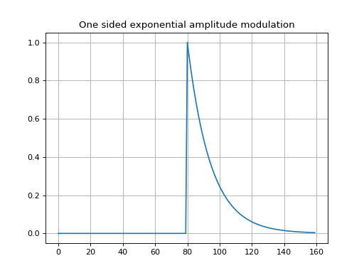
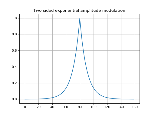
tftb.generators.amplitude_modulated.amexpos(n_points, t0=None, spread=None, kind='bilateral')[source]¶ Exponential amplitude modulation.
amexpos generates an exponential amplitude modulation starting at time t0 and spread proportioanl to spread.
Parameters: Returns: exponential function
Return type: numpy.ndarray
Examples: >>> x = amexpos(160) >>> plot(x) #doctest: +SKIP
(Source code, png, hires.png, pdf)

>>> x = amexpos(160, kind='unilateral')
>>> plot(x) #doctest: +SKIP
(Source code, png, hires.png, pdf)
-
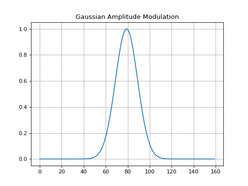
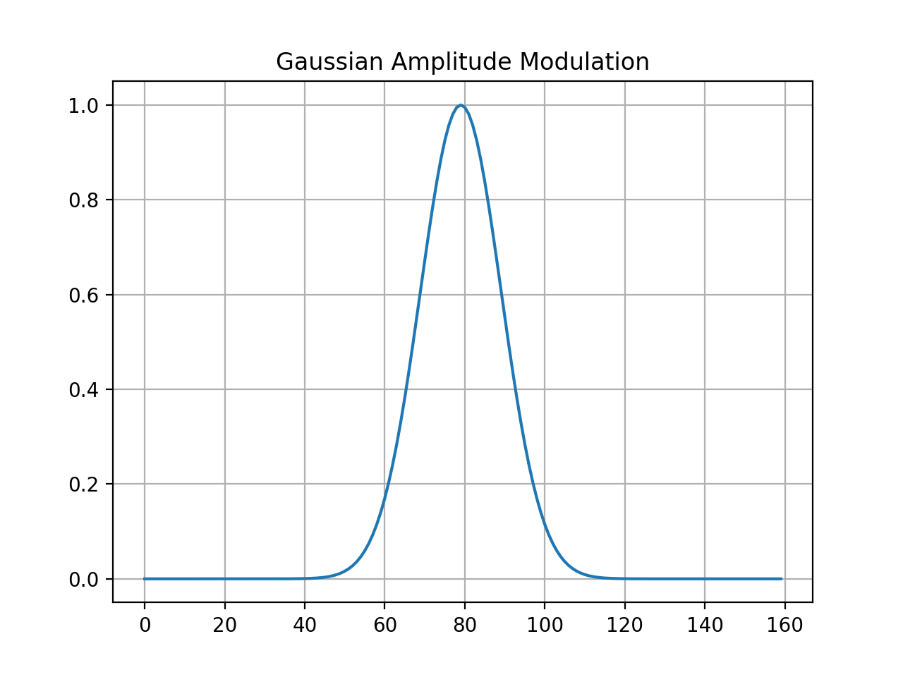
tftb.generators.amplitude_modulated.amgauss(n_points, t0=None, spread=None)[source]¶ Generate a Gaussian amplitude modulated signal.
Parameters: Returns: Gaussian function centered at time
t0.Return type: numpy.ndarray
Example: >>> x = amgauss(160) >>> plot(x) #doctest: +SKIP
(Source code, png, hires.png, pdf)

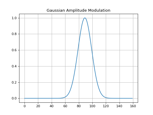
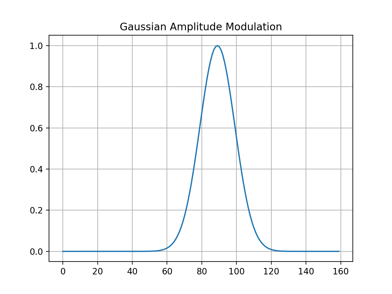
>>> x = amgauss(160, 90)
>>> plot(x) #doctest: +SKIP
(Source code, png, hires.png, pdf)

-
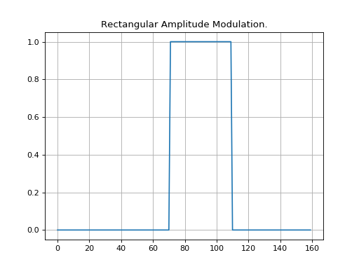
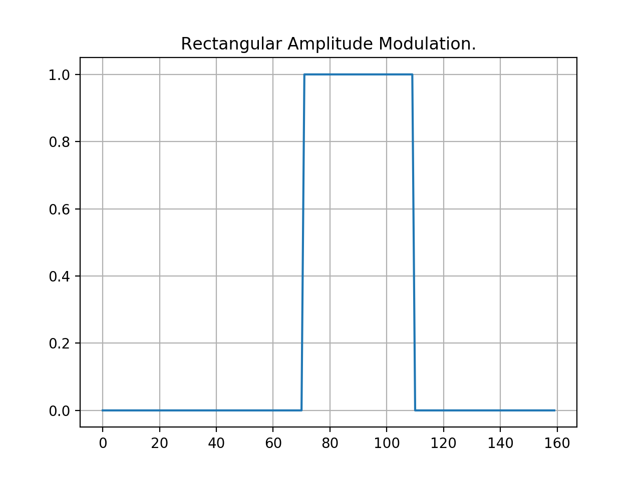
tftb.generators.amplitude_modulated.amrect(n_points, t0=None, spread=None)[source]¶ Generate a rectangular amplitude modulation.
Parameters: Returns: A rectangular amplitude modulator.
Return type: numpy.ndarray.
Examples: >>> x = amrect(160, 90, 40.0) >>> plot(x) #doctest: +SKIP
(Source code, png, hires.png, pdf)
-
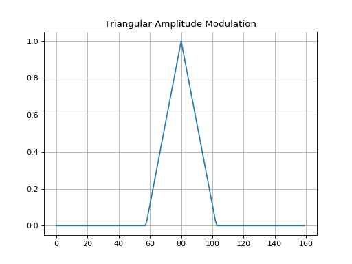
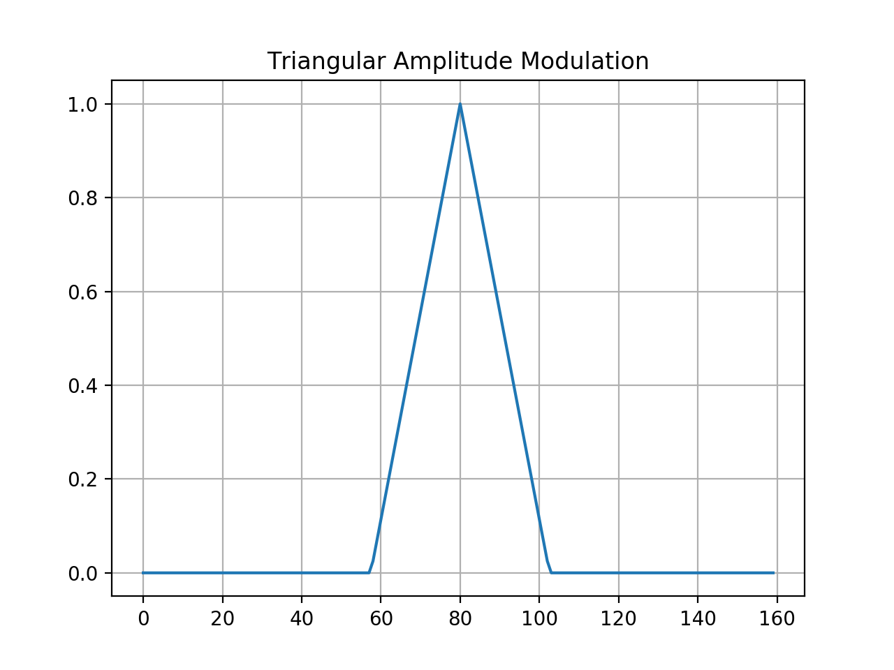
tftb.generators.amplitude_modulated.amtriang(n_points, t0=None, spread=None)[source]¶ Generate a triangular amplitude modulation.
Parameters: Returns: A triangular amplitude modulator.
Return type: numpy.ndarray.
Examples: >>> x = amtriang(160) >>> plot(x) #doctest: +SKIP
(Source code, png, hires.png, pdf)
tftb.generators.analytic_signals module
-
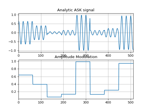
tftb.generators.analytic_signals.anaask(n_points, n_comp=None, f0=0.25)[source]¶ Generate an amplitude shift (ASK) keying signal.
Parameters: Returns: Tuple containing the modulated signal and the amplitude modulation.
Return type: tuple(numpy.ndarray)
Examples: >>> x, am = anaask(512, 64, 0.05) >>> subplot(211), plot(real(x)) #doctest: +SKIP >>> subplot(212), plot(am) #doctest: +SKIP
(Source code, png, hires.png, pdf)

-
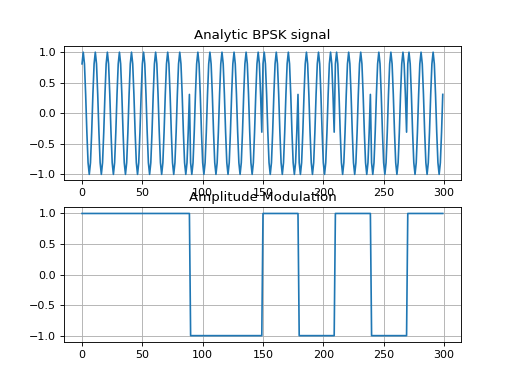
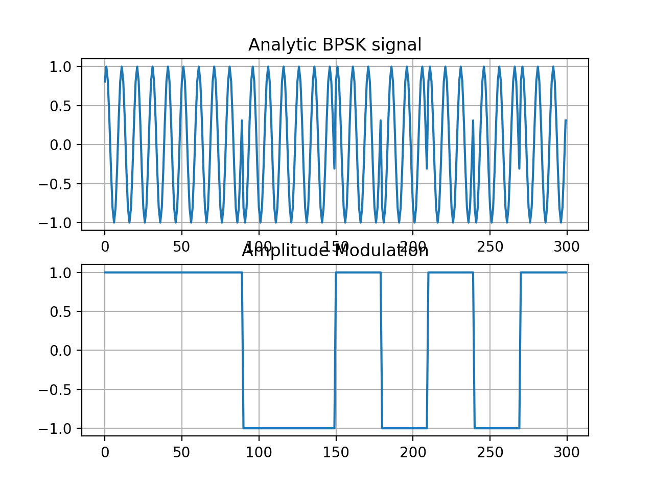
tftb.generators.analytic_signals.anabpsk(n_points, n_comp=None, f0=0.25)[source]¶ Binary phase shift keying (BPSK) signal.
Parameters: Returns: BPSK signal
Return type: numpy.ndarray
Examples: >>> x, am = anabpsk(300, 30, 0.1) >>> subplot(211), plot(real(x)) #doctest: +SKIP >>> subplot(212), plot(am) #doctest: +SKIP
(Source code, png, hires.png, pdf)

-
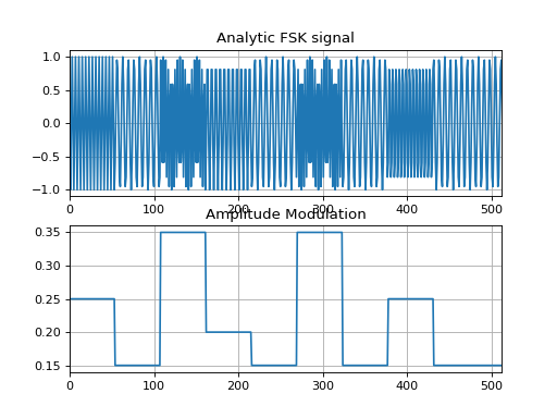
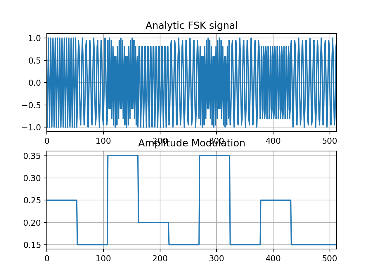
tftb.generators.analytic_signals.anafsk(n_points, n_comp=None, Nbf=4)[source]¶ Frequency shift keying (FSK) signal.
Parameters: Returns: FSK signal.
Return type: numpy.ndarray
Examples: >>> x, am = anafsk(512, 54.0, 5.0) >>> subplot(211), plot(real(x)) #doctest: +SKIP >>> subplot(212), plot(am) #doctest: +SKIP
(Source code, png, hires.png, pdf)
-
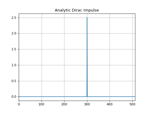
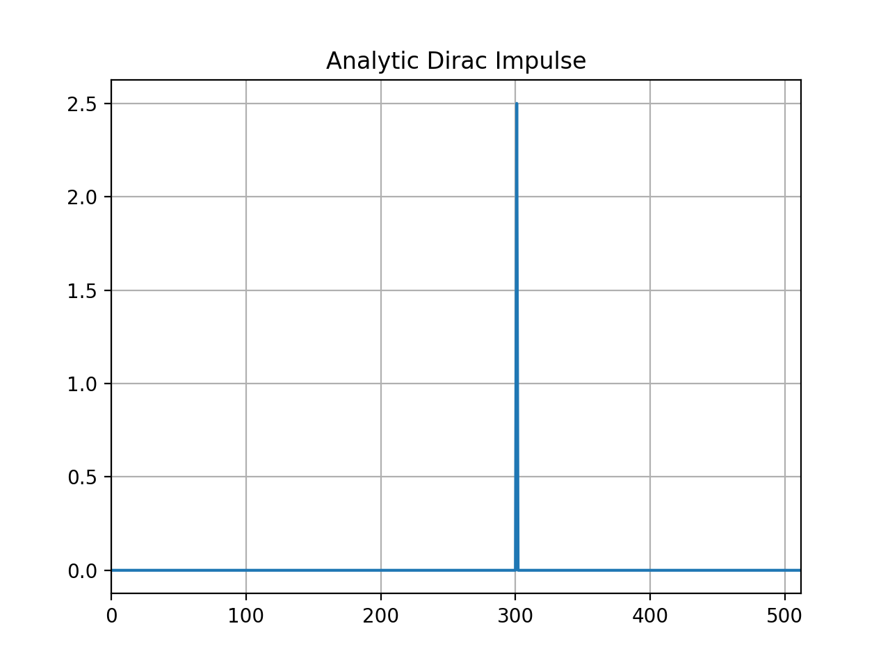
tftb.generators.analytic_signals.anapulse(n_points, ti=None)[source]¶ Analytic projection of unit amplitude impulse signal.
Parameters: Returns: analytic impulse signal.
Return type: numpy.ndarray
Examples: >>> x = 2.5 * anapulse(512, 301) >>> plot(real(x)) #doctest: +SKIP
(Source code, png, hires.png, pdf)

-
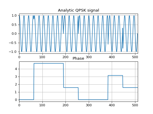
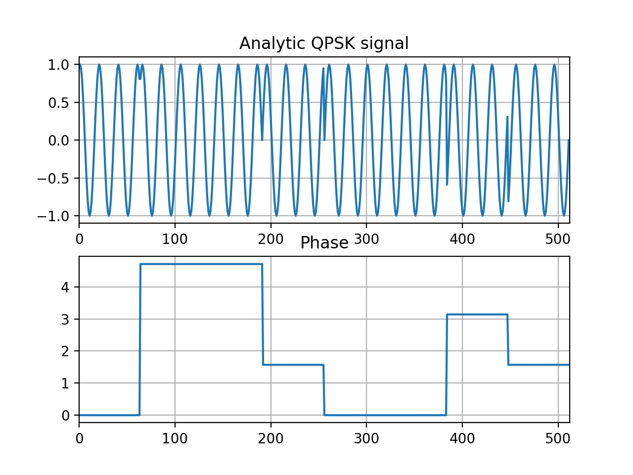
tftb.generators.analytic_signals.anaqpsk(n_points, n_comp=None, f0=0.25)[source]¶ Quaternary Phase Shift Keying (QPSK) signal.
Parameters: Returns: complex phase modulated signal of normalized frequency f0 and initial phase.
Return type: Examples: >>> x, phase = anaqpsk(512, 64.0, 0.05) >>> subplot(211), plot(real(x)) #doctest: +SKIP >>> subplot(212), plot(phase) #doctest: +SKIP
(Source code, png, hires.png, pdf)
-
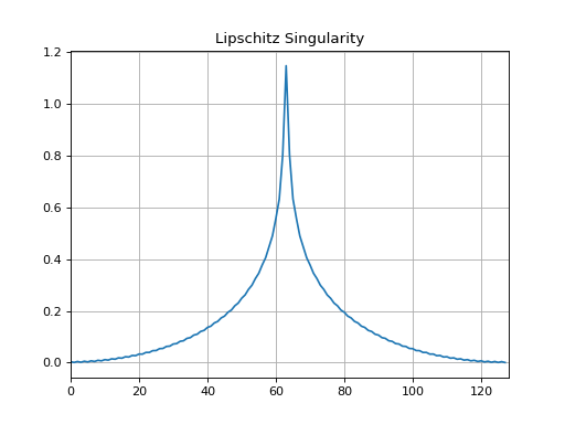
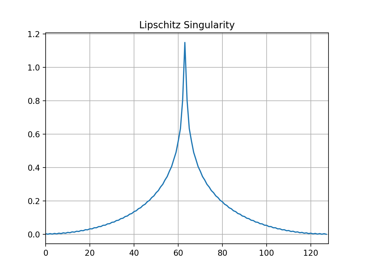
tftb.generators.analytic_signals.anasing(n_points, t0=None, h=0.0)[source]¶ Lipschitz singularity. Refer to the wiki page on Lipschitz condition, good test case.
Parameters: Returns: N-point Lipschitz singularity centered around t0
Return type: numpy.ndarray
Examples: >>> x = anasing(128) >>> plot(real(x)) #doctest: +SKIP
(Source code, png, hires.png, pdf)
tftb.generators.frequency_modulated module
-
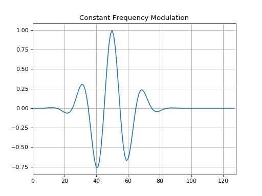
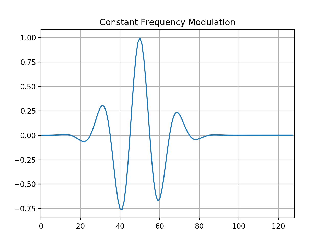
tftb.generators.frequency_modulated.fmconst(n_points, fnorm=0.25, t0=None)[source]¶ Generate a signal with constant frequency modulation.
Parameters: Returns: frequency modulation signal with frequency fnorm
Return type: numpy.ndarray
Examples: >>> from tftb.generators import amgauss >>> z = amgauss(128, 50, 30) * fmconst(128, 0.05, 50)[0] >>> plot(real(z)) #doctest: +SKIP
(Source code, png, hires.png, pdf)

-
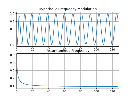
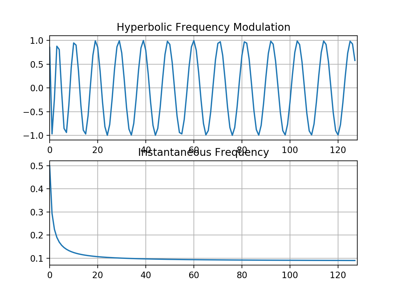
tftb.generators.frequency_modulated.fmhyp(n_points, p1, p2)[source]¶ Signal with hyperbolic frequency modulation.
Parameters: Returns: vector containing the modulated signal samples.
Return type: numpy.ndarray
Examples: >>> signal, iflaw = fmhyp(128, (1, 0.5), (32, 0.1)) >>> subplot(211), plot(real(signal)) #doctest: +SKIP >>> subplot(212), plot(iflaw) #doctest: +SKIP
(Source code, png, hires.png, pdf)

-
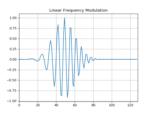
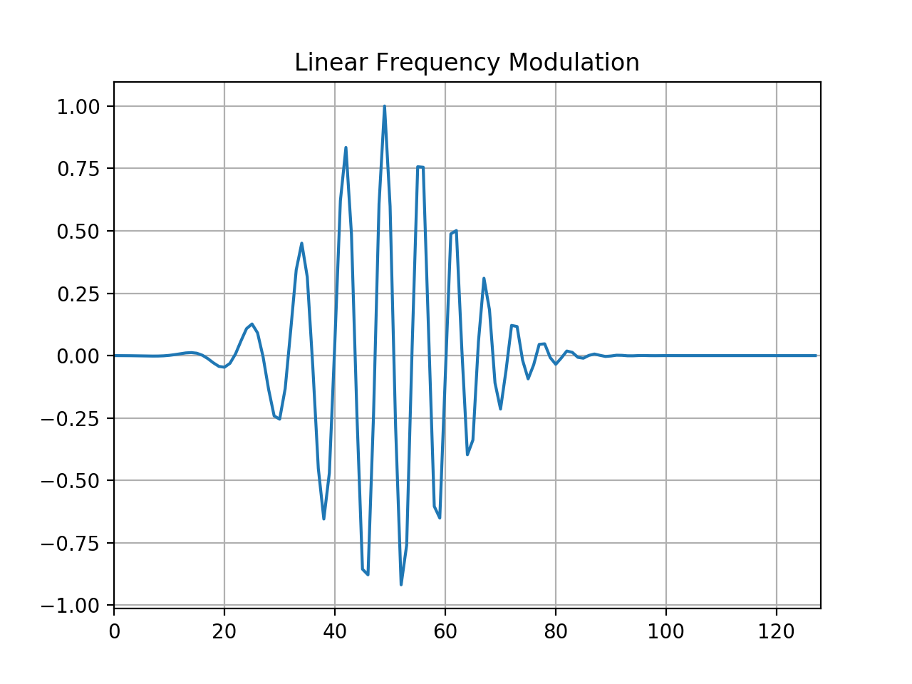
tftb.generators.frequency_modulated.fmlin(n_points, fnormi=0.0, fnormf=0.5, t0=None)[source]¶ Generate a signal with linear frequency modulation.
Parameters: Returns: The modulated signal, and the instantaneous amplitude law.
Return type: tuple(array-like)
Examples: >>> from tftb.generators import amgauss >>> z = amgauss(128, 50, 40) * fmlin(128, 0.05, 0.3, 50)[0] >>> plot(real(z)) #doctest: +SKIP
(Source code, png, hires.png, pdf)

-
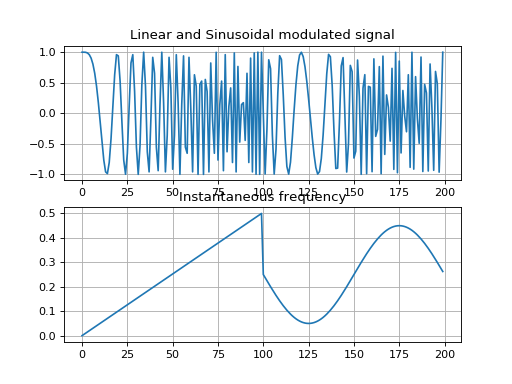
tftb.generators.frequency_modulated.fmodany(iflaw, t0=1)[source]¶ Arbitrary frequency modulation.
Parameters: - iflaw (numpy.ndarray) – Vector of instantaneous frequency law samples.
- t0 (float) – time center
Returns: output signal
Return type: Examples: >>> from tftb.generators import fmlin >>> import numpy as np >>> y1, ifl1 = fmlin(100) # A linear instantaneous frequency law. >>> y2, ifl2 = fmsin(100) # A sinusoidal instantaneous frequency law. >>> iflaw = np.append(ifl1, ifl2) # combination of the two >>> sig = fmodany(iflaw) >>> subplot(211), plot(real(sig)) #doctest: +SKIP >>> subplot(212), plot(iflaw) #doctest: +SKIP
(Source code, png, hires.png, pdf)
-
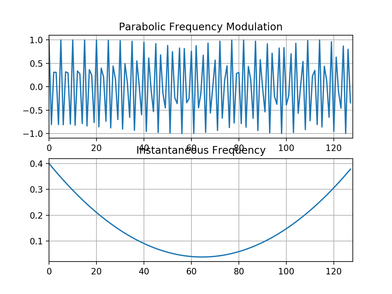
tftb.generators.frequency_modulated.fmpar(n_points, coefficients)[source]¶ Parabolic frequency modulated signal.
Parameters: Returns: Signal with parabolic frequency modulation law.
Return type: Examples: >>> x, iflaw = fmpar(128, (0.4, -0.0112, 8.6806e-05)) >>> subplot(211), plot(real(x)) #doctest: +SKIP >>> subplot(212), plot(iflaw) #doctest: +SKIP
(Source code, png, hires.png, pdf)

-
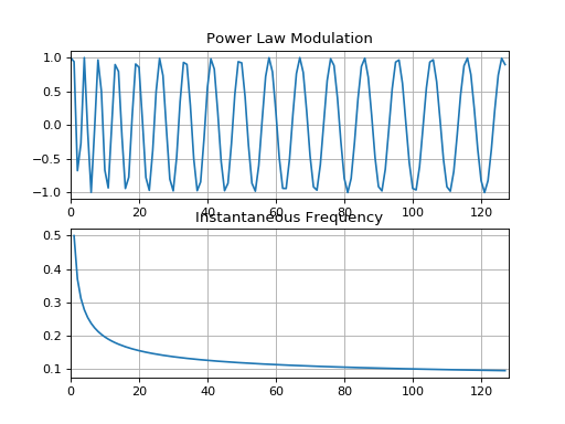
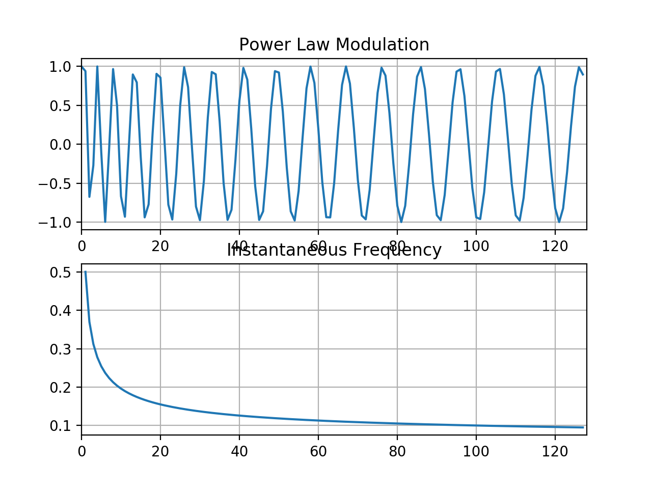
tftb.generators.frequency_modulated.fmpower(n_points, k, coefficients)[source]¶ Generate signal with power law frequency modulation.
Parameters: Returns: vector of modulated signal samples.
Return type: numpy.ndarray
Examples: >>> x, iflaw = fmpower(128, 0.5, (1, 0.5, 100, 0.1)) >>> subplot(211), plot(real(x)) #doctest: +SKIP >>> subplot(212), plot(iflaw) #doctest: +SKIP
(Source code, png, hires.png, pdf)
-
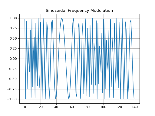
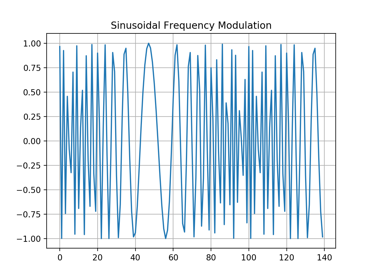
tftb.generators.frequency_modulated.fmsin(n_points, fnormin=0.05, fnormax=0.45, period=None, t0=None, fnorm0=None, pm1=1)[source]¶ Sinusodial frequency modulation.
Parameters: Returns: output signal
Return type: numpy.ndarray
Examples: >>> z = fmsin(140, period=100, t0=20, fnorm0=0.3, pm1=-1) >>> plot(real(z)) #doctest: +SKIP
(Source code, png, hires.png, pdf)
tftb.generators.misc module
-
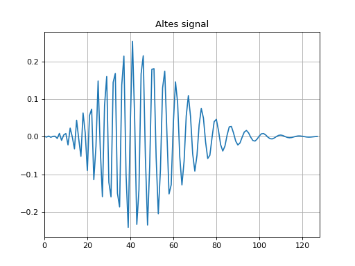
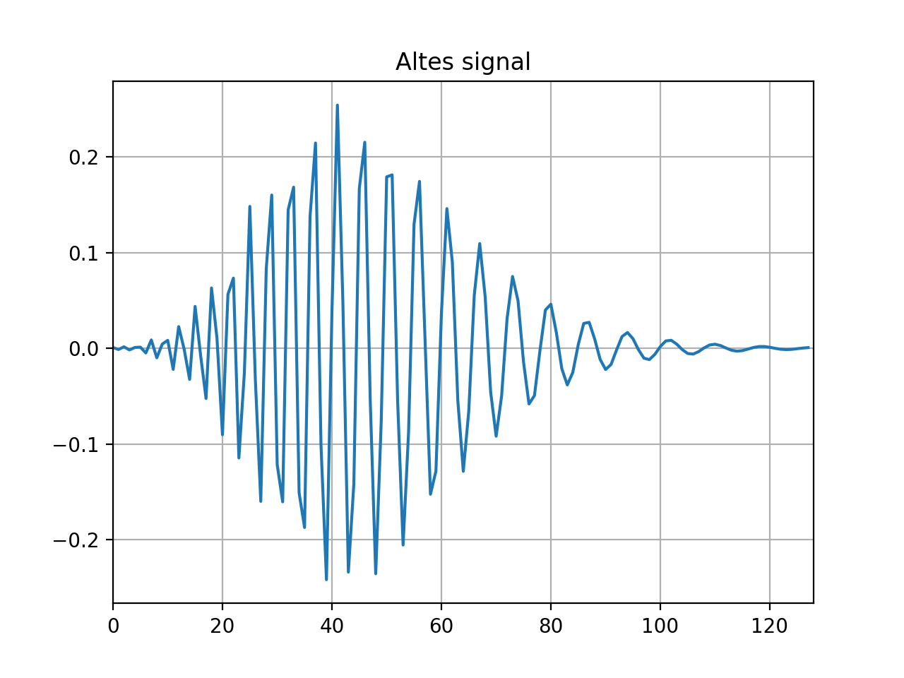
tftb.generators.misc.altes(n_points, fmin=0.05, fmax=0.5, alpha=300)[source]¶ Generate the Altes signal in time domain.
Parameters: Returns: Time vector containing the Altes signal samples.
Return type: numpy.ndarray
Examples: >>> x = altes(128, 0.1, 0.45) >>> plot(x) #doctest: +SKIP
(Source code, png, hires.png, pdf)

-
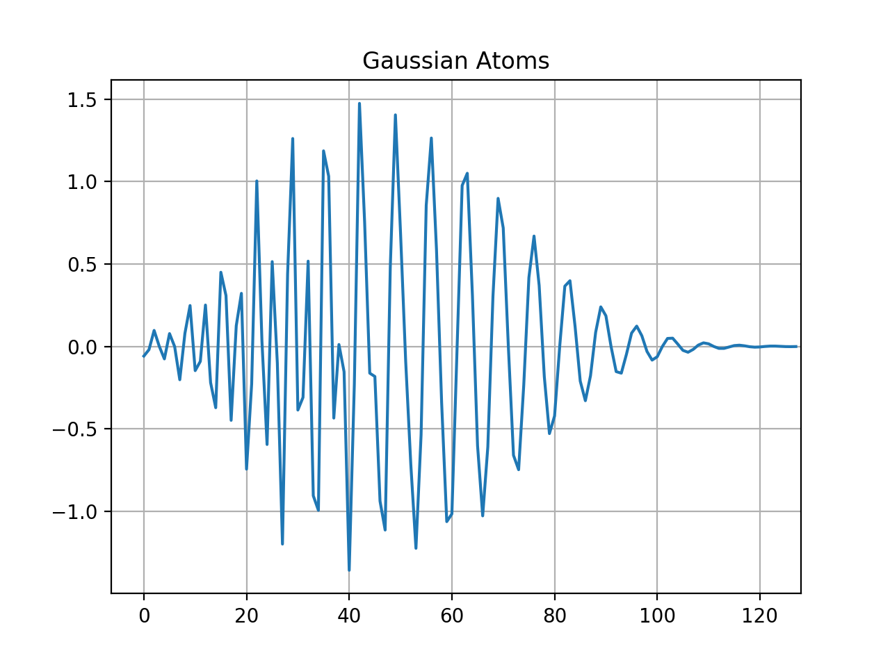
tftb.generators.misc.atoms(n_points, coordinates)[source]¶ Compute linear combination of elementary Gaussian atoms.
Parameters: - n_points (int) – Number of points in a signal
- coordinates (array-like) – matrix of time-frequency centers
Returns: signal
Return type: array-like
Examples: >>> import numpy as np >>> coordinates = np.array([[32.0, 0.3, 32.0, 1.0], [0.15, 0.15, 48.0, 1.22]]) >>> sig = atoms(128, coordinates) >>> plot(real(sig)) #doctest: +SKIP
(Source code, png, hires.png, pdf)

-
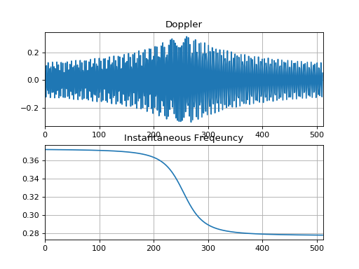
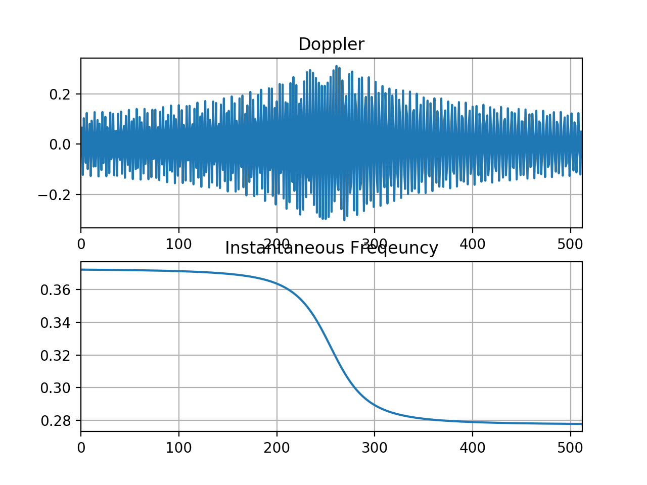
tftb.generators.misc.doppler(n_points, s_freq, f0, distance, v_target, t0=None, v_wave=340.0)[source]¶ Generate complex Doppler signal
Parameters: Returns: Tuple containing output frequency modulator, output amplitude modulator, output instantaneous frequency law.
Return type: Example: >>> fm, am, iflaw = doppler(512, 200.0, 65.0, 10.0, 50.0) >>> subplot(211), plot(real(am * fm)) #doctest: +SKIP >>> subplot(211), plot(iflaw) #doctest: +SKIP
(Source code, png, hires.png, pdf)
-
tftb.generators.misc.gdpower(n_points, degree=0.0, rate=1.0)[source]¶ Generate a signal with a power law group delay.
Parameters: Returns: Tuple of time row containing modulated samples, group delay, frequency bins.
Return type:
-
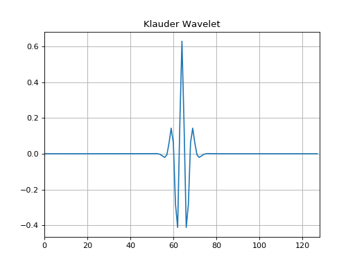
tftb.generators.misc.klauder(n_points, attenuation=10.0, f0=0.2)[source]¶ Klauder wavelet in time domain.
Parameters: Returns: Time row vector containing klauder samples.
Return type: numpy.ndarray
Example: >>> x = klauder(128) >>> plot(x) #doctest: +SKIP
(Source code, png, hires.png, pdf)

-
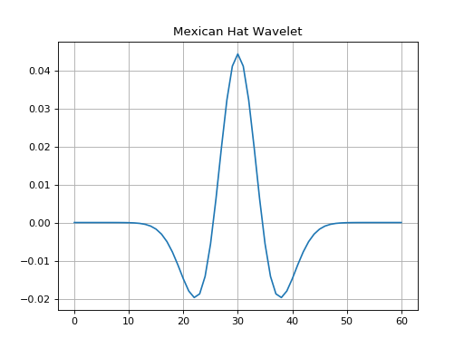
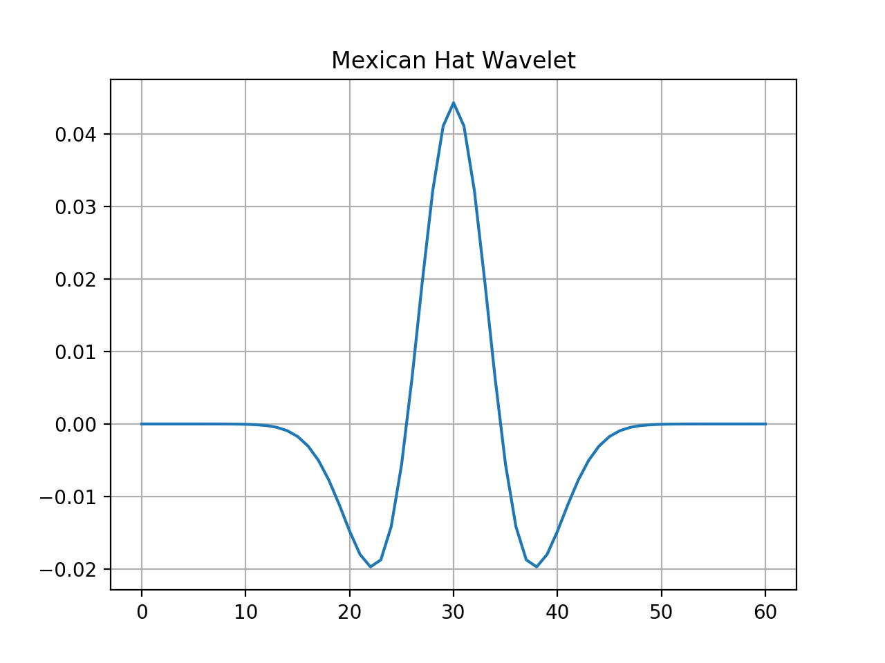
tftb.generators.misc.mexhat(nu=0.05)[source]¶ Mexican hat wavelet in time domain.
Parameters: nu (float) – Central normalized frequency of the wavelet. Must be a real number between 0 and 0.5 Returns: time vector containing mexhat samples. Return type: numpy.ndarray Example: >>> plot(mexhat()) #doctest: +SKIP
(Source code, png, hires.png, pdf)
tftb.generators.noise module
-
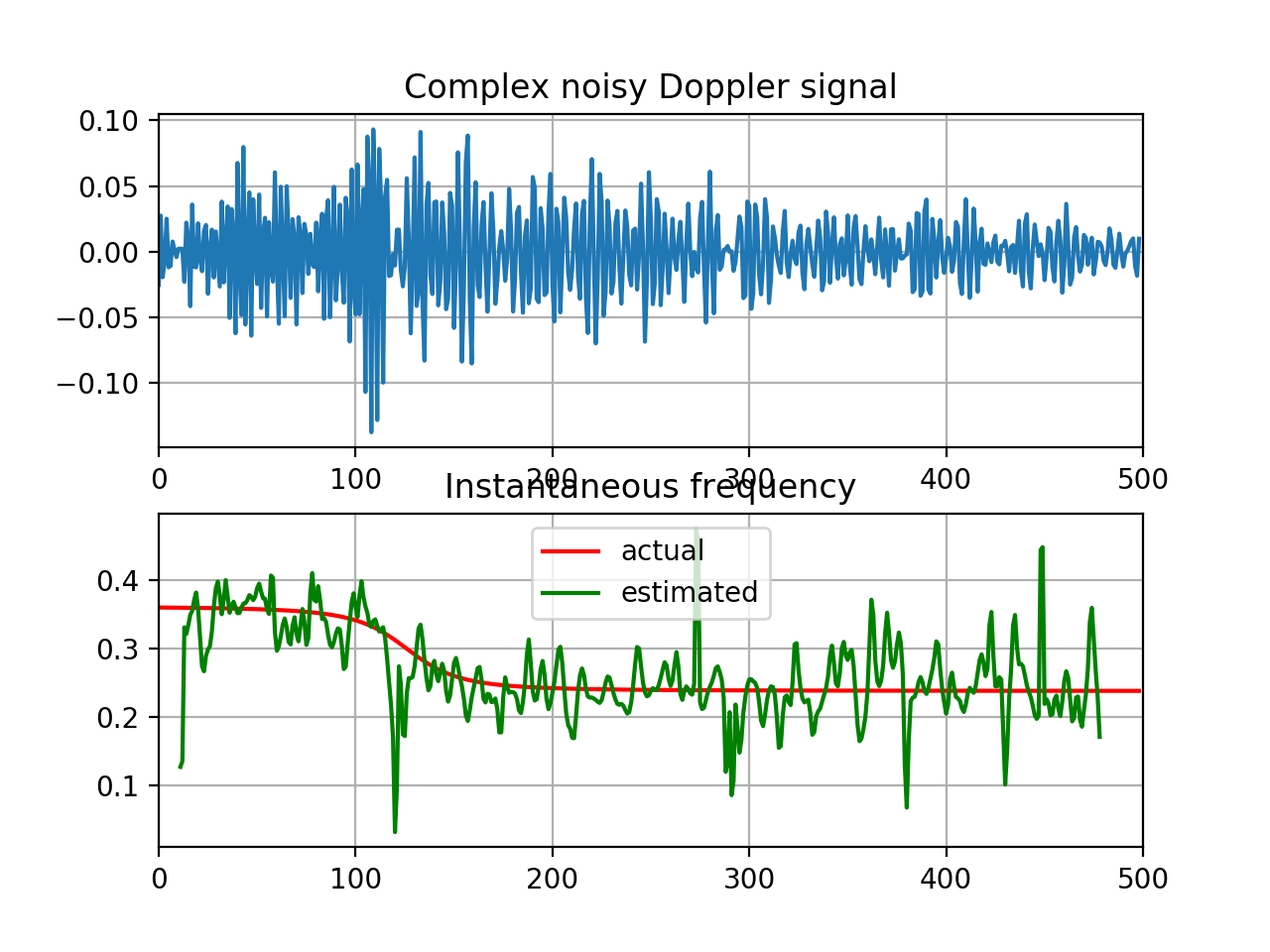
tftb.generators.noise.dopnoise(n_points, s_freq, f_target, distance, v_target, time_center=None, c=340)[source]¶ Generate complex noisy doppler signal, normalized to have unit energy.
Parameters: - n_points (int) – Number of points.
- s_freq (float) – Sampling frequency.
- f_target (float) – Frequency of target.
- distance (float) – Distnace from line to observer.
- v_target (float) – velocity of target relative to observer.
- time_center (float) – Time center. (Default n_points / 2)
- c (float) – Wave velocity (Default 340 m/s)
Returns: tuple (output signal, instantaneous frequency law.)
Return type: tuple(array-like)
Example: >>> import numpy as np >>> from tftb.processing import inst_freq >>> z, iflaw = dopnoise(500, 200.0, 60.0, 10.0, 70.0, 128.0) >>> subplot(211), plot(real(z)) #doctest: +SKIP >>> ifl = inst_freq(z, np.arange(11, 479), 10) >>> subplot(212), plot(iflaw, 'r', ifl, 'g') #doctest: +SKIP
(Source code, png, hires.png, pdf)

-
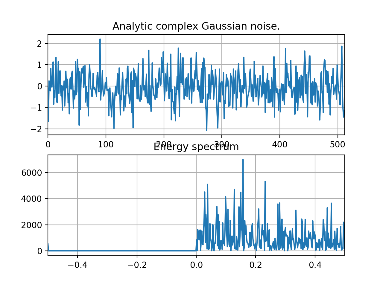
tftb.generators.noise.noisecg(n_points, a1=None, a2=None)[source]¶ Generate analytic complex gaussian noise with mean 0.0 and variance 1.0.
Parameters: Returns: Analytic complex Gaussian noise of length n_points.
Return type: numpy.ndarray
Examples: >>> import matplotlib.pyplot as plt >>> import numpy as np >>> noise = noisecg(512) >>> print("%.1f" % abs((noise ** 2).mean())) 0.0 >>> print("%.1f" % np.std(noise) ** 2) 1.0 >>> plt.subplot(211), plt.plot(real(noise)) #doctest: +SKIP >>> plt.subplot(212), #doctest: +SKIP >>> plt.plot(linspace(-0.5, 0.5, 512), abs(fftshift(fft(noise))) ** 2) #doctest: +SKIP
(Source code, png, hires.png, pdf)

-
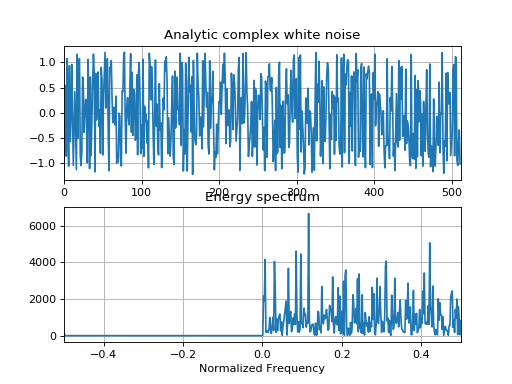
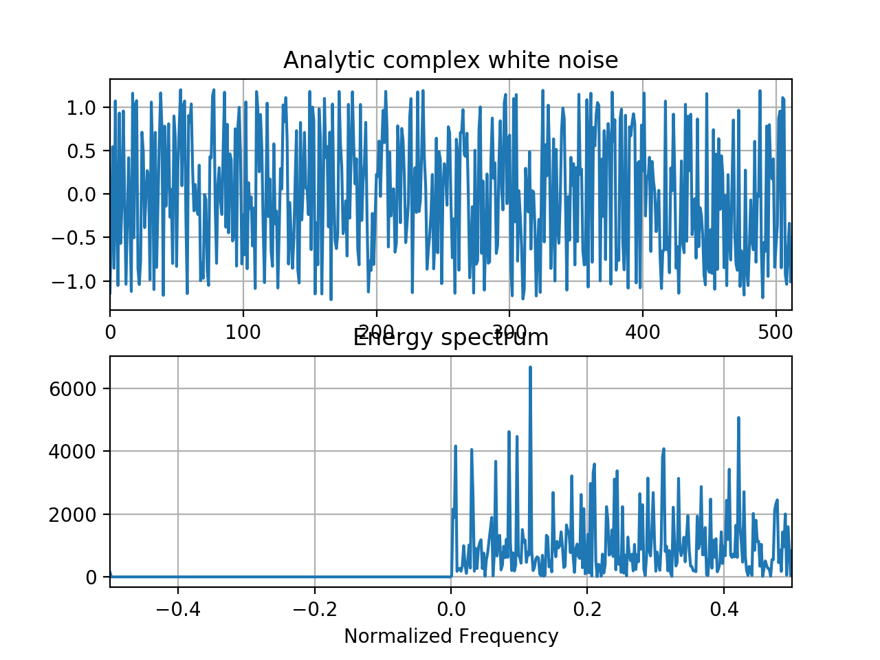
tftb.generators.noise.noisecu(n_points)[source]¶ Compute analytic complex uniform white noise.
Parameters: n_points (int) – Length of the noise signal. Returns: analytic complex uniform white noise signal of length N Return type: numpy.ndarray Examples: >>> import matplotlib.pyplot as plt >>> import numpy as np >>> noise = noisecu(512) >>> print("%.2f" % abs((noise ** 2).mean())) 0.00 >>> print("%.1f" % np.std(noise) ** 2) 1.0 >>> plt.subplot(211), plt.plot(real(noise)) #doctest: +SKIP >>> plt.subplot(212), #doctest: +SKIP >>> plt.plot(linspace(-0.5, 0.5, 512), abs(fftshift(fft(noise))) ** 2) #doctest: +SKIP
(Source code, png, hires.png, pdf)
tftb.generators.utils module
Module contents
-
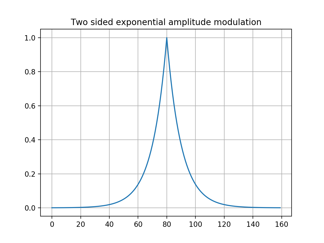
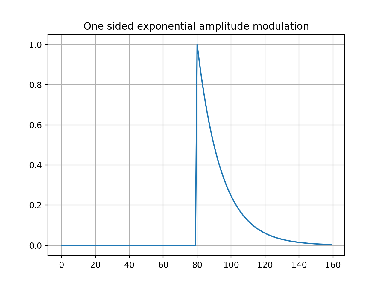
tftb.generators.amexpos(n_points, t0=None, spread=None, kind='bilateral')[source]¶ Exponential amplitude modulation.
amexpos generates an exponential amplitude modulation starting at time t0 and spread proportioanl to spread.
Parameters: Returns: exponential function
Return type: numpy.ndarray
Examples: >>> x = amexpos(160) >>> plot(x) #doctest: +SKIP
(Source code, png, hires.png, pdf)
>>> x = amexpos(160, kind='unilateral')
>>> plot(x) #doctest: +SKIP
(Source code, png, hires.png, pdf)
-
tftb.generators.amgauss(n_points, t0=None, spread=None)[source]¶ Generate a Gaussian amplitude modulated signal.
Parameters: Returns: Gaussian function centered at time
t0.Return type: numpy.ndarray
Example: >>> x = amgauss(160) >>> plot(x) #doctest: +SKIP
(Source code, png, hires.png, pdf)
>>> x = amgauss(160, 90)
>>> plot(x) #doctest: +SKIP
(Source code, png, hires.png, pdf)
-
tftb.generators.amrect(n_points, t0=None, spread=None)[source]¶ Generate a rectangular amplitude modulation.
Parameters: Returns: A rectangular amplitude modulator.
Return type: numpy.ndarray.
Examples: >>> x = amrect(160, 90, 40.0) >>> plot(x) #doctest: +SKIP
(Source code, png, hires.png, pdf)
-
tftb.generators.amtriang(n_points, t0=None, spread=None)[source]¶ Generate a triangular amplitude modulation.
Parameters: Returns: A triangular amplitude modulator.
Return type: numpy.ndarray.
Examples: >>> x = amtriang(160) >>> plot(x) #doctest: +SKIP
(Source code, png, hires.png, pdf)
-
tftb.generators.fmconst(n_points, fnorm=0.25, t0=None)[source]¶ Generate a signal with constant frequency modulation.
Parameters: Returns: frequency modulation signal with frequency fnorm
Return type: numpy.ndarray
Examples: >>> from tftb.generators import amgauss >>> z = amgauss(128, 50, 30) * fmconst(128, 0.05, 50)[0] >>> plot(real(z)) #doctest: +SKIP
(Source code, png, hires.png, pdf)
-
tftb.generators.fmhyp(n_points, p1, p2)[source]¶ Signal with hyperbolic frequency modulation.
Parameters: Returns: vector containing the modulated signal samples.
Return type: numpy.ndarray
Examples: >>> signal, iflaw = fmhyp(128, (1, 0.5), (32, 0.1)) >>> subplot(211), plot(real(signal)) #doctest: +SKIP >>> subplot(212), plot(iflaw) #doctest: +SKIP
(Source code, png, hires.png, pdf)
-
tftb.generators.fmlin(n_points, fnormi=0.0, fnormf=0.5, t0=None)[source]¶ Generate a signal with linear frequency modulation.
Parameters: Returns: The modulated signal, and the instantaneous amplitude law.
Return type: tuple(array-like)
Examples: >>> from tftb.generators import amgauss >>> z = amgauss(128, 50, 40) * fmlin(128, 0.05, 0.3, 50)[0] >>> plot(real(z)) #doctest: +SKIP
(Source code, png, hires.png, pdf)
-
tftb.generators.fmodany(iflaw, t0=1)[source]¶ Arbitrary frequency modulation.
Parameters: - iflaw (numpy.ndarray) – Vector of instantaneous frequency law samples.
- t0 (float) – time center
Returns: output signal
Return type: Examples: >>> from tftb.generators import fmlin >>> import numpy as np >>> y1, ifl1 = fmlin(100) # A linear instantaneous frequency law. >>> y2, ifl2 = fmsin(100) # A sinusoidal instantaneous frequency law. >>> iflaw = np.append(ifl1, ifl2) # combination of the two >>> sig = fmodany(iflaw) >>> subplot(211), plot(real(sig)) #doctest: +SKIP >>> subplot(212), plot(iflaw) #doctest: +SKIP
(Source code, png, hires.png, pdf)
-
tftb.generators.fmpar(n_points, coefficients)[source]¶ Parabolic frequency modulated signal.
Parameters: Returns: Signal with parabolic frequency modulation law.
Return type: Examples: >>> x, iflaw = fmpar(128, (0.4, -0.0112, 8.6806e-05)) >>> subplot(211), plot(real(x)) #doctest: +SKIP >>> subplot(212), plot(iflaw) #doctest: +SKIP
(Source code, png, hires.png, pdf)
-
tftb.generators.fmpower(n_points, k, coefficients)[source]¶ Generate signal with power law frequency modulation.
Parameters: Returns: vector of modulated signal samples.
Return type: numpy.ndarray
Examples: >>> x, iflaw = fmpower(128, 0.5, (1, 0.5, 100, 0.1)) >>> subplot(211), plot(real(x)) #doctest: +SKIP >>> subplot(212), plot(iflaw) #doctest: +SKIP
(Source code, png, hires.png, pdf)
-
tftb.generators.fmsin(n_points, fnormin=0.05, fnormax=0.45, period=None, t0=None, fnorm0=None, pm1=1)[source]¶ Sinusodial frequency modulation.
Parameters: Returns: output signal
Return type: numpy.ndarray
Examples: >>> z = fmsin(140, period=100, t0=20, fnorm0=0.3, pm1=-1) >>> plot(real(z)) #doctest: +SKIP
(Source code, png, hires.png, pdf)
-
tftb.generators.sigmerge(x1, x2, ratio=0.0)[source]¶ Add two signals with a specific energy ratio in decibels.
Parameters: - x1 (numpy.ndarray) – 1D numpy.ndarray
- x2 (numpy.ndarray) – 1D numpy.ndarray
- ratio (float) – Energy ratio in decibels.
Returns: The merged signal
Return type: numpy.ndarray
-
tftb.generators.scale(X, a, fmin, fmax, N)[source]¶ Scale a signal with the Mellin transform.
Parameters: Returns: A-scaled version of X.
Return type: array-like
-
tftb.generators.dopnoise(n_points, s_freq, f_target, distance, v_target, time_center=None, c=340)[source]¶ Generate complex noisy doppler signal, normalized to have unit energy.
Parameters: - n_points (int) – Number of points.
- s_freq (float) – Sampling frequency.
- f_target (float) – Frequency of target.
- distance (float) – Distnace from line to observer.
- v_target (float) – velocity of target relative to observer.
- time_center (float) – Time center. (Default n_points / 2)
- c (float) – Wave velocity (Default 340 m/s)
Returns: tuple (output signal, instantaneous frequency law.)
Return type: tuple(array-like)
Example: >>> import numpy as np >>> from tftb.processing import inst_freq >>> z, iflaw = dopnoise(500, 200.0, 60.0, 10.0, 70.0, 128.0) >>> subplot(211), plot(real(z)) #doctest: +SKIP >>> ifl = inst_freq(z, np.arange(11, 479), 10) >>> subplot(212), plot(iflaw, 'r', ifl, 'g') #doctest: +SKIP
(Source code, png, hires.png, pdf)
-
tftb.generators.noisecg(n_points, a1=None, a2=None)[source]¶ Generate analytic complex gaussian noise with mean 0.0 and variance 1.0.
Parameters: Returns: Analytic complex Gaussian noise of length n_points.
Return type: numpy.ndarray
Examples: >>> import matplotlib.pyplot as plt >>> import numpy as np >>> noise = noisecg(512) >>> print("%.1f" % abs((noise ** 2).mean())) 0.0 >>> print("%.1f" % np.std(noise) ** 2) 1.0 >>> plt.subplot(211), plt.plot(real(noise)) #doctest: +SKIP >>> plt.subplot(212), #doctest: +SKIP >>> plt.plot(linspace(-0.5, 0.5, 512), abs(fftshift(fft(noise))) ** 2) #doctest: +SKIP
(Source code, png, hires.png, pdf)
-
tftb.generators.noisecu(n_points)[source]¶ Compute analytic complex uniform white noise.
Parameters: n_points (int) – Length of the noise signal. Returns: analytic complex uniform white noise signal of length N Return type: numpy.ndarray Examples: >>> import matplotlib.pyplot as plt >>> import numpy as np >>> noise = noisecu(512) >>> print("%.2f" % abs((noise ** 2).mean())) 0.00 >>> print("%.1f" % np.std(noise) ** 2) 1.0 >>> plt.subplot(211), plt.plot(real(noise)) #doctest: +SKIP >>> plt.subplot(212), #doctest: +SKIP >>> plt.plot(linspace(-0.5, 0.5, 512), abs(fftshift(fft(noise))) ** 2) #doctest: +SKIP
(Source code, png, hires.png, pdf)
-
tftb.generators.anaask(n_points, n_comp=None, f0=0.25)[source]¶ Generate an amplitude shift (ASK) keying signal.
Parameters: Returns: Tuple containing the modulated signal and the amplitude modulation.
Return type: tuple(numpy.ndarray)
Examples: >>> x, am = anaask(512, 64, 0.05) >>> subplot(211), plot(real(x)) #doctest: +SKIP >>> subplot(212), plot(am) #doctest: +SKIP
(Source code, png, hires.png, pdf)
-
tftb.generators.anabpsk(n_points, n_comp=None, f0=0.25)[source]¶ Binary phase shift keying (BPSK) signal.
Parameters: Returns: BPSK signal
Return type: numpy.ndarray
Examples: >>> x, am = anabpsk(300, 30, 0.1) >>> subplot(211), plot(real(x)) #doctest: +SKIP >>> subplot(212), plot(am) #doctest: +SKIP
(Source code, png, hires.png, pdf)
-
tftb.generators.anafsk(n_points, n_comp=None, Nbf=4)[source]¶ Frequency shift keying (FSK) signal.
Parameters: Returns: FSK signal.
Return type: numpy.ndarray
Examples: >>> x, am = anafsk(512, 54.0, 5.0) >>> subplot(211), plot(real(x)) #doctest: +SKIP >>> subplot(212), plot(am) #doctest: +SKIP
(Source code, png, hires.png, pdf)
-
tftb.generators.anapulse(n_points, ti=None)[source]¶ Analytic projection of unit amplitude impulse signal.
Parameters: Returns: analytic impulse signal.
Return type: numpy.ndarray
Examples: >>> x = 2.5 * anapulse(512, 301) >>> plot(real(x)) #doctest: +SKIP
(Source code, png, hires.png, pdf)
-
tftb.generators.anaqpsk(n_points, n_comp=None, f0=0.25)[source]¶ Quaternary Phase Shift Keying (QPSK) signal.
Parameters: Returns: complex phase modulated signal of normalized frequency f0 and initial phase.
Return type: Examples: >>> x, phase = anaqpsk(512, 64.0, 0.05) >>> subplot(211), plot(real(x)) #doctest: +SKIP >>> subplot(212), plot(phase) #doctest: +SKIP
(Source code, png, hires.png, pdf)
-
tftb.generators.anasing(n_points, t0=None, h=0.0)[source]¶ Lipschitz singularity. Refer to the wiki page on Lipschitz condition, good test case.
Parameters: Returns: N-point Lipschitz singularity centered around t0
Return type: numpy.ndarray
Examples: >>> x = anasing(128) >>> plot(real(x)) #doctest: +SKIP
(Source code, png, hires.png, pdf)
-
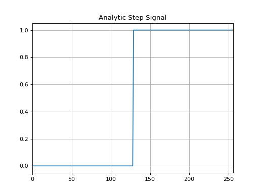
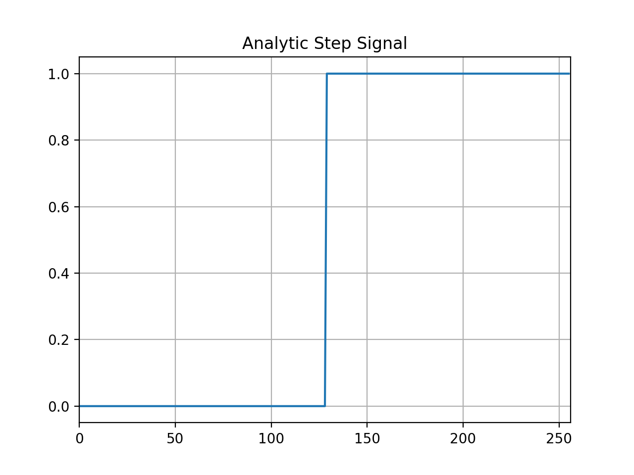
tftb.generators.anastep(n_points, ti=None)[source]¶ Analytic projection of unit step signal.
Parameters: Returns: output signal
Return type: numpy.ndarray
Examples: >>> x = anastep(256, 128) >>> plot(real(x)) #doctest: +SKIP
(Source code, png, hires.png, pdf)

-
tftb.generators.doppler(n_points, s_freq, f0, distance, v_target, t0=None, v_wave=340.0)[source]¶ Generate complex Doppler signal
Parameters: Returns: Tuple containing output frequency modulator, output amplitude modulator, output instantaneous frequency law.
Return type: Example: >>> fm, am, iflaw = doppler(512, 200.0, 65.0, 10.0, 50.0) >>> subplot(211), plot(real(am * fm)) #doctest: +SKIP >>> subplot(211), plot(iflaw) #doctest: +SKIP
(Source code, png, hires.png, pdf)
-
tftb.generators.gdpower(n_points, degree=0.0, rate=1.0)[source]¶ Generate a signal with a power law group delay.
Parameters: Returns: Tuple of time row containing modulated samples, group delay, frequency bins.
Return type:
-
tftb.generators.klauder(n_points, attenuation=10.0, f0=0.2)[source]¶ Klauder wavelet in time domain.
Parameters: Returns: Time row vector containing klauder samples.
Return type: numpy.ndarray
Example: >>> x = klauder(128) >>> plot(x) #doctest: +SKIP
(Source code, png, hires.png, pdf)
-
tftb.generators.mexhat(nu=0.05)[source]¶ Mexican hat wavelet in time domain.
Parameters: nu (float) – Central normalized frequency of the wavelet. Must be a real number between 0 and 0.5 Returns: time vector containing mexhat samples. Return type: numpy.ndarray Example: >>> plot(mexhat()) #doctest: +SKIP
(Source code, png, hires.png, pdf)
-
tftb.generators.altes(n_points, fmin=0.05, fmax=0.5, alpha=300)[source]¶ Generate the Altes signal in time domain.
Parameters: Returns: Time vector containing the Altes signal samples.
Return type: numpy.ndarray
Examples: >>> x = altes(128, 0.1, 0.45) >>> plot(x) #doctest: +SKIP
(Source code, png, hires.png, pdf)
-
tftb.generators.atoms(n_points, coordinates)[source]¶ Compute linear combination of elementary Gaussian atoms.
Parameters: - n_points (int) – Number of points in a signal
- coordinates (array-like) – matrix of time-frequency centers
Returns: signal
Return type: array-like
Examples: >>> import numpy as np >>> coordinates = np.array([[32.0, 0.3, 32.0, 1.0], [0.15, 0.15, 48.0, 1.22]]) >>> sig = atoms(128, coordinates) >>> plot(real(sig)) #doctest: +SKIP
(Source code, png, hires.png, pdf)